Using of pH as a tool to predict salinity of groundwater for irrigation purpose using artificial neural network

(1)

of groundwater for irrigation purpose

using artiﬁcial neural network

Mahmoud Nasr

a

, Hoda Farouk Zahran

b,*

a

Sanitary Engineering Department, Faculty of Engineering, Alexandria University, P.O. Box 21544, Alexandria, Egypt

b

Plant Production Department, Water Research, Arid Lands Cultivation Research Institute (ALCRI), City of Scientiﬁc Research and Technological Applications, Alexandria, Egypt

Received 10 May 2014; revised 20 June 2014; accepted 20 June 2014 Available online 25 July 2014

KEYWORDS

Groundwater;

Artiﬁcial neural network; Salinity

Abstract Monitoring of groundwater quality is one of the important tools to provide adequate information about water management. In the present study, artificial neural network (ANN) with a feed-forward back-propagation was designed to predict groundwater salinity, expressed by total dissolved solids (TDS), using pH as an input parameter. Groundwater samples were collected from a 36 m depth well located in the experimental farm of the City of Scientific Researches and Tech-nological Applications (SRTA City), New Borg El-Arab City, Alexandria, Egypt. The network structure was 1–5–3–1 and used the default Levenberg–Marquardt algorithm for training. It was observed that, the best validation performance, based on the mean square error, was 14819 at epoch 0, and no major problems or over-fitting occurred with the training step. The simulated output tracked the measured data with a correlation coefficient (R-value) of 0.64, 0.67 and 0.90 for train-ing, validation and test, respectively. In this case, the network response was acceptable, and simu-lation could be used for entering new inputs.

ª2014 Hosting by Elsevier B.V. on behalf of National Institute of Oceanography and Fisheries.

1. Introduction

In Egypt, water supply is the most important factor to be stud-ied where agriculture and industrial sectors are the essential roles in the development of human civilization (Seyyed et al., 2013). Additionally, in arid and semi-arid regions groundwater

is the major source for domestic and irrigation purposes (Zare et al., 2011). Water table is the level below the land-surface where all the voids in soil and rock are ﬁlled with water. This saturated zone is called groundwater (Podmore, 2009). Salinity is deﬁned as the equivalent Na Cl salt percentage that dis-solved with the soils coming from pollutants in rainwater. Another source of salinity is the rock weathering which causes salt that released as minerals to break down over time. As shown inFig. 1, high soil salinity levels are negatively affecting humans and the natural resources (Slinger and Tenison, 2007). Salinity is composed of hundreds of different ions, including chloride (Cl), sodium (Na+_{), nitrate (NO}

3

_{), calcium}

* Corresponding author. Tel.: +20 1227108250. E-mail address:[email protected](H.F. Zahran).

Peer review under responsibility of National Institute of Oceanography and Fisheries.

http://dx.doi.org/10.1016/j.ejar.2014.06.005

(2)

(Ca+2), magnesium (Mg+2), bicarbonate (HCO3), and sulfate

(SO4 2

). Moreover, toxic ions such as boron (B), bromide (Br) and iron (Fe) could be accumulated at higher levels (Groundwater information sheet-salinity, 2010). During irriga-tion work salinity, occurs due to the rise in saline groundwater and the build-up of salt in the soil surface of irrigated land-scapes (Podmore, 2009). As a result of ‘‘irrigation salinity’’, salts may reach levels that adversely affect plants and crop pro-duction and may result in harmful effects at high concentra-tions of toxic ions such as chloride ions. Excess of sodium ion concentrations in leaves can cause leaf burn, necrotic (dead) patches and even defoliation. Similarly, plants affected by chloride toxicity exhibit similar foliar symptoms, such as leaf bronzing and necrotic spots in some species (Podmore, 2009). Salinity of water may be estimated from a frequent surement of total dissolved solids (TDS). The TDS is a mea-sure of the total dissolved salts/substances in water, including organic and suspended particles that can pass through a very small ﬁlter (Podmore, 2009).

Recently, mathematical, statistical and computational methods to simulate and assess many aquifer water quality parameters have been investigated (Seyyed et al., 2013). Groundwater modeling has become a principal branch of many projects and studies dealing with groundwater develop-ment, protection and remediation. Moreover, modeling is a promising tool for predicting groundwater behavior based on hydrological variables (Maedeh et al., 2013). According to the modeling techniques, artificial neural network (ANN) has been established to quantify the general meaningful solutions to problems even when the input data contain errors or are uncertainty (Seyyed et al., 2013). ANN refers to computing systems whose basic theme is inspired from biological neuron processing, known as the human brain. The brain consists of large number of neurons, interconnected with each other by synapses, known as neural networks (Nasr et al., 2012). Each node receives and processes weighted input from a preceding layer and propagates its output to nodes in the subsequent neighbor through links. Previously, ANN has been used in many groundwater quality modeling. Sandhu and Finch, 1996 found that the ANN provided a fast and reasonably accurate method of modeling the relationship between flows and water quality. Moreover, this relationship was further used to estimate the Sacramento River flow required to meet a salinity standard. Moreover, Rogers and Dowla, 1994

presented a new approach to nonlinear groundwater

manage-ment methodology aimed at optimizing aquifer remediation in line with the application of ANN. Similarly, Morshed and Kaluarachchi, 1998 stated that ANN optimization methods can be used to perform inverse groundwater modeling for parameter estimation.

The objective of the present study is to build a model of ANN for studying the relation between groundwater alkalin-ity (i.e. in terms of pH) and salinalkalin-ity (i.e. expressed by TDS). After that, the developed ANN model would be applied in many practical and theoretical applications as well decision making.

2. Materials and methods

2.1. Groundwater sampling and analyses

Groundwater samples were collected from a 36 m depth well located in the experimental farm of the City of Scientiﬁc Researches and Technological Applications (SRTA), New Borg El-Arab City, Alexandria, Egypt. The samples were har-vested in summer, autumn, and winter, 2013. This period was satisfactory as it covers all probable seasonal variations in the studied variables. The gathered samples were preserved, trans-ported and analyzed according to Standard Methods for Examination of Water and Waste Water (Eaton et al., 2005). Analyses were included pH and TDS parameters.

2.2. Artiﬁcial neural network theory

Artiﬁcial neural networks are generally presented as systems of interconnected nodes which can compute values from inputs. Simple artiﬁcial nodes are class of statistical models could be called ‘‘Neural’’ if they possess the following characteristics: consist of sets of adaptive weights, i.e. numerical parameters that are tuned by a learning algorithm, and are capable of approximating non-linear functions of their inputs. The adaptive weights are conceptually connection strengths between neurons, which are activated during training and prediction (Hinton et al., 2006). The network structure is composed of a set of neurons connected by links and organized in number of layers. Each layer is fully interconnected to the preceding layer by weights (Nasr et al., 2012). Initial suggested weights are progressively adjusted during the training process by compar-ing predicted outputs with measured data (targets). The

(3)

computation of network weights and biases is known as ‘‘training step’’. The objective of the back-propagation training algorithm is to ﬁnd the optimal weights by minimizing the mean square error (MSE) of the output values (Nasr et al.,2013). Simultaneously, learning functions are used to update the layer’s weight and bias. This procedure is completed in the ‘‘validation step’’, where the network is improved to avoid data over-ﬁtting (Hong et al., 2003). After that a set of data is randomly used to examine the network generalization, i.e. the ‘‘test step’’.

Each scalar input (p) is multiplied by a scalar weight (W), and then added to a scalar bias (b), resulted in the net input (n=Wp+b). Finally, the result is passed through the trans-fer functionf, which gets the neuron’s outputa, wherea=f

(Wp+b) (Demuth et al., 2007). Those functions can be (i) lin-ear transfer functions: used in the final layer to find a linlin-ear approximation to a nonlinear function, or (ii) sigmoid transfer functions: used in the hidden layers to generate the output between 0 and 1 for Log-Sigmoid and between1 and 1 for Tan-Sigmoid, even if the input data have infinity values.

2.3. Artiﬁcial neural network applied to predict TDS

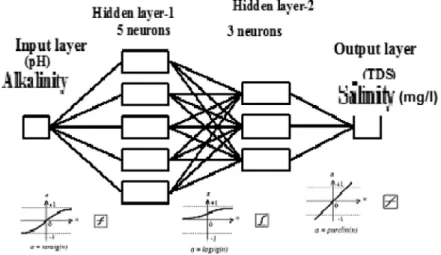
In this study a feed forward neural network (FFNN) with back-propagation training algorithm was applied to correlate the relation between input alkalinity expressed in (pH) and output salinity expressed in (TDS). The ANN configuration was identified based on a previous research by Nasr et al., 2013and through conducting several trials until reaching the best regression results with no over-fittingFig. 2. The network properties were as follows:

– Network input: pH.

– Network output: TDS concentrations.

– Network type: Feed-forward back-propagation.

– Training function: Levenberg–Marquardt algorithm (TRAINLM).

– Adaptation learning function: Gradient descent with momentum weight/bias learning function (LEARNGDM). – Performance function: Mean square error (MSE).

– Number of layers: 3 (layer-1: ﬁve neurons and TANSIG transfer function; layer-2: three neurons and LOGSIG

transfer function; output layer: PURELIN transfer function).

– Data records were randomly divided into three subsets, i.e. training: 60%, validation: 20% and test: 20%.

3. Results and discussion

3.1. Quality of water fed to artiﬁcial neural network (ANN) conﬁguration to predict TDS values

Analysis of the groundwater samples is shown inTable 1.

3.2. Artiﬁcial neural network conﬁguration applied to predict TDS

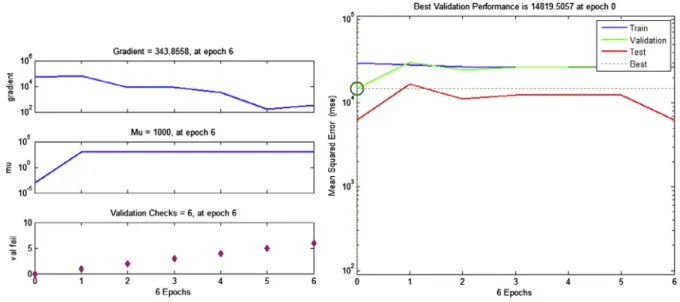
As shown in Fig. 3, the magnitude of the gradient and the number of validation checks were used to terminate the network training. At epoch: 6 iterations, the gradient was equal to 343.86 (i.e. at gradient less than 1e-5, the training will stop). The number of validation checks was equal to 6; which

Figure 2 Artiﬁcial neural network (ANN) conﬁguration applied to predict TDS value.

Table 1 Measured pH ranges and corresponding average values of TDS.

Season Ranges of pH values Average values of TDS (ppm)

Summer 7.50–7.75 4396.6 7.64–7.71 4765.8 7.68–7.40 4747.6 7.77–7.98 4808.7 7.48–7.51 4828.2 Autumn 7.60–7.66 4542.2 8.08–8.02 4644.9 8.15–8.06 4699.5 7.94–7.91 4777.5 7.97–8.13 4747.6 Winter 8.10–8.16 4656.6 7.07–7.37 4828.2 8.05–8.16 4859.4 8.02–8.13 4919.2 8.02–8.13 4934.8

(4)

is the appropriate value to stop training.1 The performance plot shows the value of the function, in terms of training, validation, and test behaviors, versus the iteration number. The best validation performance, based on the mean square error, was 14819 at epoch 0.

Since the validation and test curves are very similar, therefore no major problems or over-ﬁtting occurred with the training.

During training, each neuron in the layer adjusts its weight vector toward the closest group of input vectors. The ﬁnal weights and biases were:

Weight to layer 1 from input 1 ðwf1;1gÞ 5:08 4:06 12:46 11:31 6:63 2 6 6 6 6 6 6 6 4 3 7 7 7 7 7 7 7 5

Figure 3 Training state and performance of the generated ANN model.

1

The time consumed to complete the training progress was 0:00:06 using ‘‘nntool’’ neural network toolboxin MATLABR2014a; PC memory: 2.00 GB RAM.

(5)

Bias to layer 2ðbf2gÞ 2:55 0:97 4:64 2 6 4 3 7 5 Bias to layer 3ðbf3gÞ ½0:65

As displayed inFig. 4, a linear regression analysis was con-ducted for training, validation and testing, in order to deter-mine the relationship between the outputs of the network and the targets. In each plot, the dashed line represents the per-fect result, i.e. outputs = targets, whereas the solid line corre-sponds to the best fit linear regression. As the R-value approaches to one, then there is an exact linear relationship. The regression results (R-value) were 0.64, 0.67 and 0.90 for training, validation and test, respectively. Those results were corresponding to a total response of 0.68. The lower regression results can be attributed to fewer training data (accounting for 78 points) and/or the ANN configuration, in terms of number of hidden layers and neurons, might not being optimal. After the network was trained, validated and tested, the generated model can be used to predict the parameter TDS through new input pH data. In (Maedeh et al., 2013) a similar research, ANN was used to predict TDS variations in groundwater of Tehran. The study found R2 of 0.96 between the forecast and observed data using input parameters: SO4, Na, and Cl. Additionally,Seyyed et al., 2013revealed that it was possible to predict TDS distribution with access to input parameters such as PH and EC with a correlation coefficient of 0.96. Sim-ilarly,Nourani et al., 2013applied FFNN to predict the values of EC and TDS using inputs: temperature, pH, opacity, total hardness and quantity of calcium, and the study found a cor-relation coefficient of more than 0.90.

It was found that experimental analysis of TDS was close to the predicted data calculated from the conﬁguration and this conﬁrms the validity of this model.

Conclusions

In the present study, the groundwater salinity (i.e. in terms of TDS) based on alkalinity (i.e. expressed by pH) was predicted and ANN with a structure of 1–5–3–1 was proposed. The network showed an acceptable ability to capture the

Groundwater information sheet-salinity. March, 2010. State Water Resources Control. Board Division of Water Quality GAMA Program.

Hinton, G.E., Osindero, S., Teh, Y., 2006. A fast learning algorithm for deep belief nets. Neu. Comp. 18 (7), 1527–1554.

Hong, Y.S., Rosen, M.R., Bhamidimarri, R., 2003. Analysis of a municipal wastewater treatment plant using a neural network-based pattern analysis. Water Res. 37 (7), 1608–1618.

Maedeh, A.P., Mehrdadi, N., Bidhendi, G.N., Abyaneh, H.Z., 2013. Application of artiﬁcial neural network to predict total dissolved solids variations in groundwater of Tehran plain. Iran Int. J. Environ. Sust. 2 (1), 10–20.

Morshed, J., Kaluarachchi, J., 1998. Parameter estimation using artiﬁcial neural network and genetic algorithm for free-product migration and recovery. Water Resour. Res. 34 (5), 1101–1113. Nasr, M., Moustafa, M., Seif, H., El Kobrosy, G., 2012. Application

of Artiﬁcial Neural Network (ANN) for the prediction of EL-AGAMY wastewater treatment plant performance-EGYPT. Alex Eng J. 51(1), 37–43.

Nasr, M., Tawﬁk, A., Ookawara S., Suzuki, M., 2013. Prediction of hydrogen production using artiﬁcial neural network. Seventeenth International Water Technology Conference, IWTC17, Istanbul. Nourani, V., Khanghah, T., Sayyadi, M., 2013. Application of the

Artiﬁcial Neural Network to monitor the quality of treated water. Intern J Manag Info Techy. 3(1), 38–45.

Podmore, C., 2009. Irrigation salinity – causes and impacts. PRIME-FACT for proﬁtable, adaptive and sustainable primary industries-937. October.

Rogers, L., Dowla, F., 1994. Optimization of groundwater remedia-tion using artiﬁcial neural networks with parallel solute transport modeling. Wat Resou Res. 30(2), 457–481.

Sandhu, N., Finch, R., 1996. Emulation of DWRDSM using Artiﬁcial Neural Networks and Estimation of Sacramento River Flow from Salinity,’’ North American Water and Environment Congress & Destructive Water, American society of civil engineers (ASCE), Anaheim, California, United States.

Seyyed, A.M., Gholamm A. K., Zeynab, P., Zeynab, B., Mohammad S., 2013. Estimate the spatial distribution TDS the fusion method Geostatistics and artiﬁcial neural networks. Inter J Agric Crop Sci. 6(7), 410–420.

Slinger, D., Tenison, K., 2007. Salinity Glove Box Guide: NSW Murray & Murrumbidgee Catchments, NSW Department of Primary Industries.

Zare, A.H., V.M., Bayat, V.M., Daneshkare, A.P., 2011. Forecasting nitrate concentration in groundwater using artiﬁcial neural net-work and linear regression models. Int. Agrophys. 25, 187–192.