QUANTILE REGRESSION METHODS FOR RECURSIVE
STRUCTURAL EQUATION MODELS
Lingjie Ma
Roger Koenker
THE INSTITUTE FOR FISCAL STUDIES
DEPARTMENT OF ECONOMICS
,
UCL
STRUCTURAL EQUATION MODELS LINGJIE MA AND ROGER KOENKER
Abstract. Two classes of quantile regression estimation methods for the recursive structural equation models of Chesher (2003) are investigated. A class of weighted average derivative estimators based directly on the identification strategy of Chesher is contrasted with a new control variate estimation method. The latter imposes stronger restrictions achieving an asymptotic efficiency bound with respect to the former class. An application of the methods to the study of the effect of class size on the performance of Dutch primary school students shows that (i.) reductions in class size are beneficial for good students in language and for weaker students in mathematics, (ii) larger classes appear beneficial for weaker language students, and (iii.) the impact of class size on both mean and median performance is negligible.
1. Introduction
Classical two-stage least squares methods and the limited information maximum likelihood estimator provide attractive methods of estimation for Gaussian linear structural equation models with additive errors. However, these methods offer only a conditional mean view of the structural relationship, implicitly imposing quite restric-tive location-shift assumptions on the way that covariates are allowed to influence the conditional distributions of the endogenous variables. Quantile regression methods seek to broaden this view, offering a more complete characterization of the stochas-tic relationship among variables and providing more robust, and consequently more efficient, estimates in some non-Gaussian settings.
Amemiya (1982) was the first to seriously consider quantile regression methods for the structural equation model showing the consistency and asymptotic normality of a class of two-stage median regression estimators. Subsequent work of Powell (1983) and Chen and Portnoy (1996) extended this approach, but maintained the focus primarily on the conditional median problem. Recent work has sought to broaden the perspective. Abadie, Angrist and Imbens (2002) considered quantile regression methods for estimating endogenous treatment effects focusing on the binary treat-ment case. Sakata (2000) has considered a median regression analogue of the LIML estimator. Chernozhukov and Hansen (2001) have proposed a novel instrumental variables approach.
Version: February 3, 2004. The authors would like to express their appreciation to Andrew Chesher for stimulating conversations regarding this work. They would also like to thank Annelie van der Wind for her extensive help with the interpretation of the PRIMA data. This work was partially supported by NSF Grant SES-0240781.
In a series of recent papers Chesher (2001, 2002, 2003) has considerably expanded the scope of quantile regression methods for structural econometric models. He con-siders a general nonlinear specification whose crucial feature is its triangular sto-chastic structure. By recursively conditioning, a sequence of conditional quantile functions are available to characterize the model and identify the structural effects. The approach may be viewed as a natural generalization of the “causal chain” models advocated by Strotz and Wold (1960). Imbens and Newey (2002) have also recently stressed the utility of the triangular stochastic structure.
Chesher has elegantly laid out the structural interpretation of his proposed mod-els and dealt with the ensuing identification issues. In so doing he has clarified the objectives of estimating models with heterogeneous structural effects; his focus on structural derivatives of conditional quantile functions provides a natural target for nonparametric identification and estimation. Our objective is to consider more prag-matic problems of estimation and inference in parametric structural models. We will consider two general classes of the estimation methods. The first is a class of av-erage derivative methods based directly on the Chesher identification strategy. The second is a new “control variate” approach. In parametric settings we compare the asymptotic behavior of the two approaches and show that the control variate meth-ods attain an efficiency bound corresponding to an optimally weighted form of the average derivative estimator. In typical applications where the precise specification of the covariate effects are subject to dispute the two estimation strategies are useful complements, offering a valuable framework for inference.
The next section introduces the recursive structural model and describes the two classes of estimators. We will focus primarily on a simple two equation setting, with some brief remarks on the extension to larger models. Sections 3 and 4 are devoted to the asymptotic behavior of the estimators and their asymptotic relative efficiency. Section 5 reports the results of a small simulation experiment designed to explore the finite sample performance of the two approaches. Section 6 describes an application of the models to the problem of estimating structural effects of changes in class size on student performance in Dutch primary schools.
2. Recursive Structural Models and Their Estimation
To motivate Chesher’s approach it is worthwhile to briefly reconsider the simple, exactly identified, triangular model,
(2.1) Yi1 =Yi2α1+x > i α2 +νi1+λνi2 (2.2) Yi2=ziβ1+x > i β2 +νi2.
Suppose that the unobserved errors νi1 and νi2 are stochastically independent and
identically distributed with νi1 ∼F1 and νi2 ∼ F2. Assume further that the νij’s are
independent of (zi, x>
i )
>
We will focus on the estimate of the scalar structural parameter α1. The classical
two stage least squares estimator of α1 may be written as,
ˆ α1 = ( ˆY > 2 MXYˆ2) −1ˆ Y2>MXY1 where ˆY2 =zβˆ1+Xβˆ2, βˆ1 = (z0MXz) −1z0 MXY2, ˆβ2 = (X0MzX)−1X0MzY2,Mz =I− z(z0 z)−1z0 , andMX =I−X(X 0 X)−1X0
. A somewhat less conventional interpretation
of ˆα1 can be derived substituting for νi2 in (2.1) to obtain
(2.3) Y1 =Y2(α1+λ)−zβ1λ+X(α2−λβ2) +ν1 ≡W δ+ν1, where W = [Y2...z...X] and δ= (δ1, δ2, δ>3) > = (α1+λ,−β1λ, α>2 −λβ > 2 ) > .
Now, suppose we estimate the hybrid structural equation (2.3) by ordinary least squares. We have the following result.
Proposition 1. αˆ1 = ˆδ1+ ˆβ −1 1 δˆ2, where δˆ= (W 0 W)−1 W0 Y1.
The proof of this result is somewhat involved and is, therefore, relegated to the Appendix, as are proofs of subsequent results, but its interpretation is simple and straightforward. The two stage least squares estimator may be viewed as a bias corrected form of the least squares estimator of the structural effect in the hybrid model (2.3).
The same strategy can be employed to estimate the conditional quantile effects in this model. We have the conditional quantile functions
Q1(τ1|Y2, z, x) = Y2(α1+λ)−zβ1λ+x>(α2−λβ2) +F1−1(τ1) Q2(τ2|x, z) = zβ1+x>β2+F2−1(τ2).
Provided that ∇zQ2(τ2|z, x) =β1 6= 0 we may write following Chesher (2003),
α1 = ∇Y2Q1(τ1|Y2, x, z) + ∇zQ1(τ1|Y2, x, z) ∇zQ2(τ2|x, z) α2 = ∇xQ1(τ1|Y2, x, z)−∇ zQ1(τ1|Y2, x, z) ∇zQ2(τ2|x, z) ∇ xQ2(τ2|x, z),
adopting the convention that Q1(τ1|Y2, x, z) is always evaluated at Y2 =Q2(τ2|x, z).
In this case, because the covariate effects take the simple location shift form, the
structural parameters α1 and α2 are globally constant independent of τ1 and τ2 and
of the exogenous variables x and z. As we will now see, this is highly unusual.
2.1. Quantile Treatment Effects for Recursive Structural Models. Now
con-sider the nonlinear recursive model
(2.4) Yi1 =ϕ1(Yi2, xi, νi1, νi2)
(2.5) Yi2 =ϕ2(zi, xi, νi2)
where as earlier we assume that νi1 and νi2 are independent, and identically
dis-tributed with νij ∼ Fj. The pairs (νi1, νi2) are also maintained to be independent of
(zi, x>
i )
>
respect to Y2 and x, and ϕ2 is assumed strictly monotonic in ν2, and differentiable
with respect to both z and x. Under these conditions, we can write the conditional
quantile functions, Q1(τ1|Q2(τ2|x, z), x) = ϕ1(Q2(τ2|x, z), x, F −1 1 (τ1), F −1 2 (τ2)) Q2(τ2|x, z) = ϕ2(z, x, F −1 2 (τ2)).
How should we measure the effect of Y2 onY1 in this model? Given the stochastic
character of the “treatment”, Y2, we must evaluate the treatment effect at various
quantiles of the treatment distribution. We may view this as corresponding to a
thought experiment in which we exogenously alter not the value ofY2as we would with
a treatment fully under our control, but instead alter the distribution of Y2. Thus,
for example, in our anticipated study of class-size effects on educational performance, we may imagine altering the prevailing distribution of class-sizes and exploring the consequences of this perturbation on various quantiles of the distribution of students’
attainment. Of course, in the model Y2 is determined according to (2.5), so to assume
otherwise requires some sort of “willing suspension of disbelief” in the model. But this is inevitable in structural models and we are always entitled to interpret effects
as long as they can be formulated in terms of well-posed gedankan experiments.
In their (infamous) tryptych on causal chain systems Strotz and Wold (1960) illus-trate this point with a vivid fresh water example:
Supposezis a vector whose various elements are the amounts of various
fish feeds (different insects, weeds, etc.) available in a given lake. The reduced form
y0
=B−1Γz0
+B−1u
would tell us specifically how the number of fish of any species depends
upon the availabilities of different feeds. The coefficient of anyz is the
partial derivative of a species population with respect to a food supply. It is to be noted, however, that the reduced form tells us nothing about the interactions among the various fish populations – it does not tell us the extent to which one species of fish feeds on another species. Those
are the causal relations among the y’s.
Suppose, in another situation, we continuously restock the lake with
species g, increasing yg by any desired amount. How will this affect
the values of the other y’s? If the system were recursive and we had
estimates of the elements of B, we would simply strike the gth
equa-tion out of the model and regard yg, the number of fish of species g, as exogenous – as a food supply or, when appearing with a negative coefficient as a poison. (pp. 421-2, emphasis added)
Recursive conditioning enables us to contemplate similar kinds of policy exper-iments in the context of the triangular structural models considered by Chesher; related models have also been recently considered by Imbens and Newey (2002). In contrast to the linear structural models of the Cowles Commission era, whose causal
effects were restricted to take the form of location shifts of the conditional distribu-tions of the endogenous variables, recent work poses the identification of structural effects in a general non-parametric framework so structural effects can take quite het-erogeneous forms. We will focus on a more restricted finite dimensional parametric formulation, a formulation that is more conducive to our asymptotic analysis. Exten-sions to sequences of models with the parametric dimension tending to infinity could be considered in subsequent work.
To explore this further, consider the following model in which Y2 exerts both a
location and a scale shift effect on Y1;
(2.6) Yi1 =Yi2α1+x
>
i α2+δYi2(νi1+λνi2)
(2.7) Yi2 =ziβ1+x
>
i β2+γziνi2.
Maintaining our prior assumptions on (νi1, νi2), and assuming thatδ 6= 0 andγ 6= 0,
we can again substitute for νi2 in (2.6) to obtain,
Yi1 =Yi2(α1+δνi1−δβ1λ/γ) +x > i α2+ Y2 i2 zi δλ γ − Yi2x > i zi δλβ2 γ , Yi2 =zi(β1+γνi2) +x > i β2.
So we have the conditional quantile functions,
Q1(τ1|Yi2, xi, zi) = Yi2θ1(τ1) +x>i θ2(τ1) + Y2 i2 zi θ3(τ1) + Yi2x>i zi θ4(τ1) (2.8) Q2(τ2|x, z) = zβ(τ2) +x > β2(τ2), (2.9) whereθ1(τ1) =α1+δF −1 1 (τ1)−δβ1λ/γ,θ2(τ1) = α2,θ3(τ1) =δλ/γ,θ4(τ1) =−δλβ2/γ, β1(τ2) = β1 +γF −1
2 (τ2) and β1(τ2) = β2. By recursive conditioning we have the
conditional quantile functions,
Q1(τ1|Q2(τ2|x, z), x, z) = Q2(τ2|x, z)(α1+δ(F1−1(τ1) +λF2−1(τ2))) +x>α2 Q2(τ2|x, z) = z(β1+γF2−1(τ2)) +x>β2
so the structural effect of interest is,
π1(τ1, τ2) = α1+δ(F
−1
1 (τ1) +λF
−1
2 (τ2)).
A straightforward calculation shows that
π1(τ1, τ2) =∇Y2Q1(τ1|Y2, x, z) + ∇z
Q1(τ1|Y2, x, z)
∇zQ2(τ2|x, z)
.
As in the location-shift model, this structural effect is independent of the
condition-ing covariates xi and zi so the Chesher identification strategy suggests an obvious
estimation strategy. Note however, that since estimation of the conditional quantile functions (2.8) and (2.9) will fail to produce the convenient cancellation of the exact calculation, some scheme to average over the covariate space would be required to obtain the structural effect. This will be even more apparent in the next subsection where a more general nonlinear-in-parameters model is considered.
Given the separate contributions of F1−1(τ1) andF
−1
2 (τ2), it is clear that π(τ1, τ2)
reflects not only the fact that the stochastic effect of Y2 on Y1 arises from two
dis-tinct sources, but also provides structural insight into how these sources are related.
Suppose we fix τ1 so ν1 is fixed at its τ1 quantile, changes in τ2 in π1(τ1, τ2) reflect
how the distribution of ν2 affects the τ1 quantile of the response Y1. On the other
hand, if we fix τ2, and allow τ1 to change, this sheds light on how the τ2 quantile of
Y2 influences the whole distribution of the response Y1. By considering variation in
both τ1 and τ2 we obtain a panoramic view of the stochastic relationship between Y2
and Y1.
Recalling that integrating the quantile function F−1
X (τ) of a random variable, X,
over the domain [0,1], yields its expectation, that is,
EX =
Z 1
0 F−1
X (t)dt,
we can define a mean quantile treatment effect by integrating out τ2, and denoting
µi =Eνi, ¯ π1(τ1) = Z 1 0 (α1+δ(F −1 1 (τ1) +λF −1 2 (τ2)))dτ2 ≡α1+δF −1 1 (τ1) +δλµ2
Averaging again, this time with respect to τ1 yields the mean treatment effect
¯ π1 = Z 1 0 (α1 +δF −1 1 (τ1) +δλµ2)dτ1 ≡α1+δµ1+δλµ2.
This mean treatment effect would be what is estimated by the two stage least squares estimator in the pure location shift version of the model, but when the effects are more heterogeneous as in this location-scale shift model the structural quantile
treat-ment effect π1(τ1, τ2) represents a deconstruction the mean effect into its
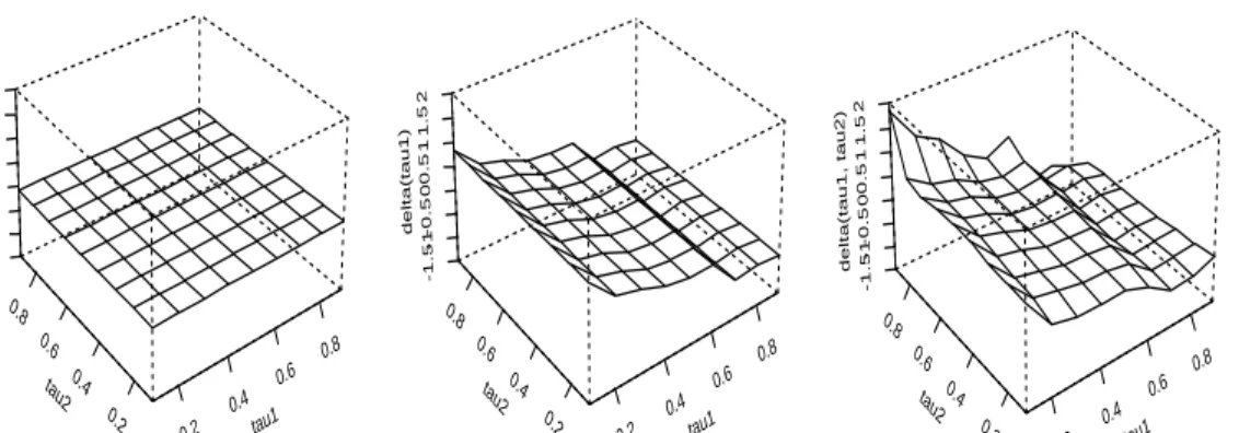
elemen-tary components. Figure 2.1 illustrates the three versions of the treatment effect
π1(τ1, τ2),π¯1(τ1) and ¯π1 for a particular parametric instance of the model (2.6-7).
2.2. Estimation of Structural Quantile Treatment Effects. In this section we
will describe two general classes of estimators for the parametric recursive structural model,
Yi1 = ϕ1(Yi2, xi, νi1, νi2;α)
(2.10)
Yi2 = ϕ2(zi, xi, νi2;β).
(2.11)
We will maintain our assumptions on the νij’s and the functions ϕ1 ϕ2 and we will
explicitly assume that the functionsϕ1 and ϕ2 are known up to the finite dimensional
parameter vectors α and β. Under these conditions we have an inverse function for
ϕ2 with respect toν2, say ˜ϕ2, allowing us to write
νi2 = ˜ϕ2(Yi2, zi, xi;β)
and thus we have,
0.2 0.4 0.6 0.8 tau1 0.2 0.4 0.6 0.8 tau2 -5 0 5 10 15 20 25 a1
Mean Treatment Effect
0.2 0.4 0.6 0.8 tau1 0.2 0.4 0.6 0.8 tau2 -5 0 5 10 15 20 25 a1(tau1)
Mean Quantile Treatment Effect
0.2 0.4 0.6 0.8 tau1 0.2 0.4 0.6 0.8 tau2 -5 0 5 10 15 20 25 a1(tau1, tau2)
Quantile Treatment Effect
Figure 2.1. Quantile Treatment Effects for the Structural Model: The figure illustrate three different notions of the structural treatment effect for the linear location-scale structural equation model: (2.6-7) with (α1, α2, δ, λ) = (10,4,3,2), (β1, β2, γ) = (1,2,3), ν1 ∼ N(0,1), ν2 ∼
N(0,0.5). The left figure depicts ¯π1 =10, the mean treatment effect; the
middle figure shows ¯π1(τ1) = 10+3F
−1
1 (τ1), the mean quantile treatment
effect; the right figure shows π1(τ1, τ2) = 10 + 3(F
−1
1 (τ1) + 2F
−1
2 (τ2)),
the general quantile treatment effect.
We will write the conditional quantile functions of Y1 and Y2 as,
Q1(τ1|Yi2, xi, zi) = h1(Yi2, xi, zi;θ) Q2(τ2|zi, xi) = h2(zi, xi;β).
Fixingτ1 and τ2 we can estimate the parameters of the conditional quantile functions,
θ(τ1) andβ(τ2), as illustrated in the previous subsection, by solving the possibly
nonlinear weighted quantile regression problems, ˆ θ(τ1) = argmin θ∈Θ n X i=1 σi1ρτ1(Yi1−h1(Yi2, xi, zi;θ)) (2.12) ˆ β(τ2) = argmin β∈B n X i=1
σi2ρτ2(Yi2−h2(zi, xi, β)).
(2.13)
The weights σij are assumed to be strictly positive and will play an important role in
the efficiency comparisons made in Section 4. The function ρτ(u) =u(τ −I(u <0))
is as in Koenker and Bassett (1978). Methods for computing quantile regression estimates for models that are nonlinear in parameters are described in Koenker and
Park (1996). When h1 and h2 yield specifications that are nonlinear in parameters,
then we require compact domains Θ and B for the parameters.
Our primary objective will be to estimate the weighted average quantile treatment effect implied by the Chesher formula,
π1(τ1, τ2) = Z ∇yQ1(τ1|y, xi, zi) + ∇z Q1(τ1|y, xi, zi) ∇zQ2(τ2|xi, zi) w(x, z)dxdz
with y evaluated as before, at Q2(τ2|xi, zi). A secondary object will be to estimate
the corresponding structural effect of the exogonous variables x,
π2(τ1, τ2) = Z ∇xQ1(τ1|Yi2, xi, zi)− ∇ zQ1(τ1|y, xi, zi) ∇zQ2(τ2|xi, zi) ∇ xQ2(τ2|xi, zi) w(x, z)dxdz
Since, in general, the above integrands depend upon the point of evaluation in the space of the exogenous covariates we consider the class of weighted average derivative estimators, ˆ π1(τ1, τ2) = n X i=1 wi ( ∇yhˆ1(τ1|y, xi, zi,θˆ) + ∇z ˆ h1(τ1|y, xi, zi,θˆ) ∇zˆh2(τ2|xi, zi.βˆ) )
again evaluating at y = ˆh2(τ2|xi, zi,βˆ). A weighted average derivative estimator for
the structural effects of x is defined similarly as,
ˆ π2(τ1, τ2) = n X i=1 wi ( ∇xhˆ1(τ1|y, xi, zi,θˆ)−∇z ˆ h1(τ1|y, xi, zi,θˆ) ∇zˆh2(τ2|xi, zi,βˆ) ∇xhˆ2(τ2|xi, zi,βˆ) ) .
The weights are assumed to be positive and sum to one. A convenient choice would
be wi ≡ n−1
. In some cases, like the location shift model the dependence on the exogenous covariates vanishes so the weights are irrelevant. The foregoing consid-erations have presumed a situation of exact identification in which there is a single
“instrumental variable,” z, available. In over-identified settings we may have several
versions of ˆπ(τ1, τ2) corresponding to different choices of the variable z and we may
wish to again consider weighted averages. This point will be addressed in more detail when we come to asymptotics.
The estimator ˆπn(τ1, τ2) = (ˆπ1(τ1, τ2),πˆ2>(τ1, τ2))> is based squarely on Chesher’s
identification strategy. Its advantage is that it takes a rather skeptical attitude toward the original model and is thereby based on a rather loosely restricted form of the two conditional quantile functions. This complements nicely the more restrictive form of the estimators described in the next subsection and consequently may eventually prove to be advantageous from a specification diagnostics and testing viewpoint.
2.3. A Control Variate Estimator. To motivate the control variate approach to
estimation of the structural quantile treatment effect, it is helpful to return briefly to the classical two stage least squares estimator of the location shift model (2.1-2)
and recall its control variate interpretation. Suppose that rather than replacingY2 by
ˆ
Y2 in (2.1) and estimating the resulting model by least squares, we instead compute
ˆ
ν2 =Y2−Yˆ2, the residuals from the first stage of 2SLS. Now consider including ˆν2 as
an additional covariate in (2.1) and estimating by least squares. It is easy to show
that the resulting estimates of α1 and α2 are the same as those produced by 2SLS.
This result holds much more generally: Yi2andzi may be vector-valued and the model
may be overidentified. A definitive original reference for this equivalence is however difficult to identify, see for example, Blundell and Powell (2003).
To apply the control variate approach to the estimation of the structural quantile
treatment effect we must first estimate the conditional τ2 quantile function of Y2 to
recover an estimate of ν2(τ2) =ν2−F2−1(τ2). Let
Q1(τ1|Yi2, xi, νi2(τ2)) =g1(Yi2, xi, νi2(τ2);α(τ1, τ2)) Q2(τ2|zi, xi) =g2(zi, xi;β(τ2))
denote the conditional quantile functions of the response variables conditioning on
the control variate, νi2(τ2). Solving
ˆ
β(τ2) = argmin
β∈B
X
σi2ρτ2(Yi2−g2(zi, xi;β))
our conditions on ϕ2 insure that we can invert to obtain the function
ν2 = ˜ϕ2(Y2, z, x, β)
so
F2−1(τ2) = ˜ϕ2(g2(z, x;β), z, x;β)
and we have ˆ
νi2(τ2) = ˜ϕ2(Yi2, zi, xi; ˆβ)−ϕ˜2(g2(zi, xi; ˆβ), zi, xi; ˆβ).
Note that the above procedure is valid regardless of the dimension of zi, so as long
as the model is identifiable ˆνi2(τ2) incorporates information on all of the available
instruments. But it does so in a much more parsimonious fashion than by introducing
zi directly into what we have referred to as the hybrid form of the first structural
equation.
Once ˆνi2(τ2) is available we can estimate the parameters of the first structural
equation by reexpressing ϕ1 as
g1(Yi2, xi,νiˆ2(τ2);a) =ϕ1(Yi2, xi, F
−1
1 (τ1),νiˆ2(τ2);α)
absorbing F1−1(τ1) into the new parameter vector a, and solving,
ˆ α(τ1, τ2) = argmin a∈A n X i=1
σi1ρτ1(Yi1−g1(Yi2, xi,νiˆ2(τ2);a)).
In the next section we will investigate the asymptotic behavior of this control variate estimator and compare its asymptotic performance with the weighted average derivative estimator. Before doing so we might remark that the restrictions imposed by the control variate procedure avoid the considerable complications of the weighted average derivative method apparent in the location-scale model (2.6-7).
2.4. Extension to m Equations. As shown by Chesher (2003) there are no real impediments to the extension of the recursive structural model to more than two equations, except some obvious notational ones. Maintaining the triangular structure
we may consider the system of m structural equations,
Y1 = ϕ1(Y2, ..., Ym, z, ν1, ..., νm, α1) Y2 = ϕ2(Y3, ..., Ym, z, ν2, ..., νm, α2)
.. .
Ym = ϕm(z, νm, αm).
The ν’s are assumed stochastically independent and independent of the exogonous
variables, z. Again, we can recursively condition to obtain the conditional quantile
functions of the Y’s and this leads to a natural generalization of the weighted average
derivative estimators. Chesher (2003) describes the exclusion restrictions and other conditions required for identification in this case.
Similarly, we can adapt the control variate estimation method to the multiple equation setting. The estimation strategy is a quite straightforward extension of the two equation situation. Starting with the last equation we estimate the control
variate ˆνm(τm) and substitute it into the (m−1)th equation, thus obtaining the control
variate ˆνm−1(τm−1), and so forth. The asymptotic representation also generalizes in
a straightforward fashion so that for the first equation, for example, we obtain a sum
of m independent terms in the Bahadur representation.
3. Asymptopia
The asymptotic behavior of the estimators described in the previous section can be developed with the aid of existing results on the asymptotics of nonlinear (in parame-ters) quantile regression estimation. We will maintain the conditions set out following the general model specification (2.4) and (2.5) and its parametric formulation (2.10) and (2.11). In addition we will employ the following regularity conditions: as, e.g., in Oberhofer (1982) and Jureˇckov´a and Proch´azka(1994).
A.1: The conditional distribution functions FY1(y1|Yi2, xi, zi) and FY2(y2|zi, xi)
are absolutely continuous with continuous densities fi1 and fi2 that are
uni-formly bounded away from 0 and∞at the pointsξi1 =Q1(τ1|Q2(τ2|zi, xi), xi, zi)
and ξi2 =Q2(τ2|zi, xi), fori = 1, . . . , n. The weights σij are positive and
uni-formly bounded away from 0 and ∞.
A.2: There exist positive definite matrices J1,J¯1, J2,J¯2 such that
lim n→∞n −1X σ2ijhij˙ h˙>ij =Jj, lim n→∞n −1X
σijfij(ξij) ˙hijh˙>ij = ¯Jj,
where ˙hi1 =∇θhi1 and ˙hi2 =∇βhi2.
A.4: There exist constants l1, l2, u1, u2 and an integer n0 > 0 such that for (θj, θ0 j)⊂Θ, (βj, β 0 j)⊂ B, j = 1,2 and n > n0, l1 kθ−θ 0 k ≤ (n−1X(h1(Yi2, xi, zi, θ)−h1(Yi2, xi, zi, θ 0 )2)1/2 ≤u1 kθ−θ 0 k l2 kβ−β 0
k ≤ (n−1X(h2(xi, zi, β)−h2(xi, zi, β
0
)2)1/2 ≤u2 kβ−β
0
k.
Theorem 1. For the parametric model (2.10-11) satisfying conditions A.1-4, the
weighted average derivative estimator πnˆ (τ1, τ2) has the asymptotic linear (Bahadur) representation √ n(ˆπn(τ1, τ2)−π(τ1, τ2)) = W1J¯1−1n −1/2 n X i=1 σi1hi˙ 1ψτ1(Yi1−ξi1) + W2J¯ −1 2 n −1/2 n X i=1 σi2hi˙ 2ψτ2(Yi2−ξi2) +op(1) ; N(0, ω11W1J¯ −1 1 J1J¯ −1 1 W > 1 +ω22W2J¯ −1 2 J2J¯ −1 2 W > 2 ) where ωjj =τj(1−τj), W1 =∇θπ(τ1, τ2) and W2 =∇βπ(τ1, τ2).
Remark: It is immediately apparent that the optimal choice of the weights, σij
involves settingσij =fij(ξij). In this case the sandwich form of the limiting covariance
matrix simplifies, and we have √ n(ˆπn(τ1, τ2)−π(τ1, τ2));N(0, ω11W1J −1 1 W > 1 +ω22W2J −1 2 W > 2 ).
Newey and Powell (1990) have shown that this density weighting achieves a semi-parametric efficiency bound for a class of linear quantile regression models. We will not address the somewhat delicate issues involved in estimating weights, but the interested reader could consult Koenker and Zhao (1994) and/or Zhao (2001).
Example: Recall that in the pure location shift version of the model (2.1-2) the
structural effect π1(τ1, τ2) is a constant α1. In this case we have model (2.1-2) and
√
n( ˆα1(τ1, τ2)−α1) is asymptotically Gaussian with mean 0 and variance
v = τ1(1−τ1) f2 1(ξ1) +λ2τ2(1−τ2) f2 2(ξ2) v−1 0 where v0 = limn→∞n −1 β0 1Z 0 MXZβ1, and MX = I −X(X 0 X)−1 X0 . The parameter
λ may be interpreted as a degree of endogeneity of the model, so the second term
in v may be viewed as a performance penalty for this endogeneity effect. It may
be noted that under these special conditions the estimator ˆα1(τ1, τ2) is equivalent
to the so-called two-stage quantile regression estimator which replaces Y2 in (2.1)
by ˆY2(τ2) the fitted values in the τ2 quantile regression estimate of (2.2) and then
estimates the τ1 quantile regression of Y1 on ˆY2(τ2) and x. A special case of this
procedure is Amemiya’s two stage least absolute deviations estimator. To the best of our knowledge no general analysis of its asymptotic behavior has been undertaken although it has been employed in several empirical studies.
To study the asymptotic behavior of the control variate estimators we require a slightly modified version of our previous regularity conditions.
B.1: The conditional distribution functions FYi1|Yi2,xi,νi2 and FYi2|zi,xi are
abso-lutely continuous with continuous densities fi1 and fi2 uniformly bounded
away from 0 and ∞ at the points ξi1 = Q1(τ1|Yi2, zi, xi), xi, ν(τ2)) and ξi2 =
Q2(τ2|zi, xi), respectively for i= 1,2, . . . , n. The weights σij are positive and
uniformly bounded away from 0 and ∞.
B.2: There exist positive definite matrices D1,D¯1, D2,D¯2 such that
lim n→∞n −1X σ2ijgij˙ g˙ > ij =Dj, lim n→∞n −1X
σijfij(ξij) ˙gijg˙ij>= ¯Dj,
where ˙gi1 =∇αgi1 and ˙gi2 =∇βgi2.
B.3: maxi=1,...,n kgij˙ k/√n→0, j = 1,2.
B.4: There exist constants l1, l2, u1, u2 and an integer n0 > 0 such that such
that, for α, α0 ∈ A,β, β0 ∈ B and n > n0, l1||α−α0|| ≤(n−1 n X i=1
(g1(Yi2, xi, νi2(τ2), α)−g1(Yi2, xi, νi2(τ2), α0))2)1/2 ≤u1||α−α0||
l2||β−β 0 || ≤(n−1 n X i=1
(g2(xi, zi, β)−g2(xi, zi, β))2)1/2 ≤u2||β−β
0
||.
These conditions are the natural analogues of our previous conditions. It may be noted that in contrast to the prior conditions, however, the possibility of overiden-tification is now permitted by the modified conditions. We can now describe the asymptotic behavior of the control variate estimator.
Theorem 2. For the parametric model (2.10-11) satisfying conditions B.1-4, the
con-trol variate estimator αˆn(τ1, τ2) has the asymptotic linear (Bahadur) representation,
√ n( ˆαn(τ1, τ2)−α(τ1, τ2)) = D¯ −1 1 n −1/2 n X i=1 σi1gi˙1ψτ1(Yi1−ξi1) + D¯−1 1 D¯12D¯−21n −1/2 n X i=1 σi2gi˙ 2ψτ2(Yi2−ξi2) +op(1) ; N(0, ω11D¯1−1D1D¯−11+ω22D¯1−1D¯12D¯2−1D2D¯2−1D¯ > 12D¯ −1 1 ) where D¯12= limn→∞n−1Pσi1fi1ηigi˙1g˙>i2 and ηi = (∂g1i/∂νi2(τ2))(∇νi2ϕi2)
−1.
Remark: Again, we see that the choice of the weights σij =fij(ξij) is optimal. It
may appear that the use of symbols σij for the weights for both classes of estimators
is an abuse of notation, but careful examination of the conditioning reveals that the conditional densities are identical in conditions A.1 and B.1 so this economy is justified at least in the two cases of primary interest: weights identically equal to one, and optimally weighted estimation according to the conditional densities.
For purposes of inference it is crucial that we have not only the marginal distribution
τ1’s and τ2’s. But this follows immediately from the Bahadur representation of the
preceding theorem.
Corollary 1. Let T1 = {τ11, ...τ1q} and T2 = {τ21, ...τ2r} with elements τij ∈ (0,1), then under the conditions of Theorem 2, the joint asymptotic distribution of{αnˆ (τ1, τ2) : τ1 ∈ T1, τ2 ∈ T2} is Gaussian with typical covariance block,
Acov √nαˆ(τ1, τ2), √nαˆ(τ3, τ4) =ω13D¯ −1 1 D13D¯ −1 3 +ω24D¯ −1 1 D¯12D¯ −1 2 D24D¯ −1 4 D¯ > 34D¯ −1 3 , where Drs= limn→∞n−1Pin=1σirσisgir˙ g˙is>, ωrs = min{τr, τs}−τrτs, with {τ1, τ3} ⊂ T1
and {τ2, τ4} ⊂ T2.
4. Asymptotic Relative Efficiency of the Structural Estimators
Naturally, we would like to compare the performance of our two classes of estima-tors. The first and most obvious prerequisite for this is to ensure that they are really estimating the same quantity. For linear in parameters specifications the situation is quite straightforward so we will consider this case in some detail first, treating it as a rehearsal for the general result embodied in Theorem 4. To formalize what we mean by linear models, suppose that
ϕ1(Yi2, xi, νi2, α, F −1 1 (τ1)) = ˙g > i1α(τ1, τ2) = ˙h > i1θ(τ1) (4.1) ϕ2(zi, xi, F −1 2 (τ2), β) = ˙g > i2β(τ2) = ˙h > i2β(τ2) (4.2)
where the vectors ˙gij and ˙hij are free of dependence on the parameters. The linearity
of ϕ1 implies that there is a linear mapping, W1 =∂π/∂θ, such that
W1θ =π.
Writing Gj for the matrix with typical row n−1/2
(fijg˙>
ij) for j = 1,2, and similarly
let Hj denote the matrix with typical row n−1/2
(fijh˙>
ij). Note that G2 = H2 and
that there is a matrix A such that G1 =H1A so Aα =θ. Thus we have W1Aα =π.
Further, let L=W1A, so Lα=π. The transformation L reduces the dimensionality
of the αvector, eliminating the components that are required to describe theν2-effect
and allowing us to focus attention on the performance of the control variate estimator
of the π parameter.
We can now compare the performance of our two estimators of π: the weighted
average derivative estimator ˆπn and the control variate estimator ˜πn=Lαnˆ . To
facil-itate this comparison it is convenient to restrict attention to the optimally weighted
form of both estimators for which σij =fij. In this case, the asymptotic covariance
matrix of ˆπn specializes to Avar(√nπnˆ ) =ω11W1J −1 1 W > 1 +ω22W2J −1 2 W > 2
while that of ˆαn specializes to
Avar(√nαnˆ ) =ω11D −1 1 +ω22D −1 1 D12D −1 2 D12D −1 1
where Di−1 = limn→∞n−1Pfij2gij˙ g˙ij> and D12 = limn→∞n−1Pfi21ηigi˙ 1g˙i>2.
Equiva-lently, we can write,
Avar(√nαnˆ ) = ω11(G > 1G1) −1 +ω22(G > 1G1) −1 G1PG2G > 1(G > 1G1) −1
where PG generically denotes the projection G(G>
G)−1
G>
onto the column space of
the matrix G. Thus, ˜π=Lαˆ, we have,
Avar(√nπ˜) = ω11L(G > 1G1) −1 L>+ω22L(G > 1G1) −1 G1PG2G > 1(G > 1G1) −1 L> Note that L(G> 1G1) −1L> = W1A(A > H> 1H1A) −1A> W> 1 = W1J1−1H > 1 H1A(A>H1>H1A)−1AH1>H1J1−1W > 1 = W1J1−1H > 1 PG1H1J −1 1 W > 1 ≤ W1J −1 1 W > 1 ,
where≤signifies the conventional ordering of matrices in the sense of positive definite
differences. Similarly, we have,
L(G>1G1) −1 G1PG2G > 1(G > 1G1) −1 L> ≤W2J −1 2 W > 2 ,
so we have established that the control variate estimator, ˜πn, has smaller asymptotic
variance than the weighted average derivative estimator ˆπn.
The efficiency advantage of the control variate estimator clearly derives from the
more restricted form of the estimator. While the restricted form of the ˜πn estimator
yields an efficiency gain when we are confident about the model specification, it clearly offers some disadvantages in situations in which we are not so confident. Indeed, tests
of model specification based on the unrestricted form of the estimators ( ˆθn,βnˆ ) might
be viewed as a reasonable precaution in the early stages of model construction. When the model is nonlinear in parameters the situation is much the same from
an asymptotic viewpoint. Jacobians of the nonlinear transformations, W1, A, and L
evaluated at the true parameters now play the role of the matrices in the previous
development, and the δ-method yields the following general result.
Theorem 3. For the parametric model (2.4-5) with the optimal weighting,σij =fij,
let Λ(α) = π denote the mapping from the structural parameter α to the weighted av-erage derivative parameter π. Suppose that the Jacobian, L=∂Λ/∂α is continuous in a neighborhood of the true parameters. Then the optimally-weighted average deriva-tive estimator, πnˆ , and the optimally-weighted control variate estimator, πn˜ = Λ( ˆαn), have limiting Gaussian behavior with asymptotic covariance matrices:
Avar(√nπnˆ ) =ω11W1J −1 1 W > 1 +ω22W2J −1 2 W > 2 Avar(√nπ˜) = ω11L(G > 1G1) −1 L>+ω22L(G > 1G1) −1 G1PG2G > 1(G > 1G1) −1 L> and Avar(√nπn˜ )≤Avar(√nπˆ).
Remark: It is worth emphasizing at this point that the superior asymptotic
when the model is overidentified. In such cases the weighted average derivative ap-proach becomes somewhat cumbersome, while the control variate method remains entirely straightforward.
5. Monte-Carlo
In this section we very briefly report on some simulation experiments designed to evaluate the performance of the estimation methods considered above. The com-putational results reported in this and the following section were carried out in the R language, Ihaka and Gentleman (1996) using the quantile regression package of Koenker (1998).
We consider a simple location-scale shift model:
Y1 = α1+α2x+ (α3+δ(λν2+ν1))Y2
(5.1)
Y2 = β1+β2x+β3z+ν2
(5.2)
where x, z, ν1 and ν2 are generated as the following: x ∼ t3, z ∼ N(15,22),
ν1 ∼ N(0,1). and ν2 ∼ N(0,0.52), We specify the parameter vectors as following,
(α1, α2, α3, δ, λ) = (3,4,4,5,3), and (β1, β2, β3) = (1,2,3). For this model, both
the weighted average derivative (WAD) and the control variate (CV) estimators for
the structural quantile treatment effect of Y2 on Y1 will converge to the population
value of 4 + 15F−1
ν2 (τ2) + 5F
−1
ν1 (τ1). For the sake of simplicity, we set τ1 = τ2 = τ
and consider only the quantiles τ = (0.1,0.3,0.5,0.7,0.9). Results are reported in
Table 5.1 for sample size n = 100, and in Table 5.2 for n = 1000. The number of
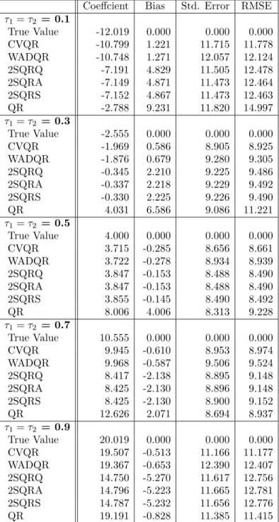
replications is R= 1000. We see first, that both estimators exhibit very modest bias
at sample size, n = 100, and bias is substantially reduced atn = 1000. Secondly, in
terms of the standard error and root mean square error, the control variate estimator outperforms the weighted derivative estimator at all considered quantiles.
For the sake of comparison we consider four other estimators:
QR: Naive quantile regression applied to (5.1) without any attempt to deal with
the endogoneity of Y2.
2SQRQ: Two stage quantile regression replacing Y2 by the predicted ˆY2 from
the τ =τ2 quantile regression estimation of (5.2).
2SQRA: Two stage quantile regression replacing Y2 by the predicted ˆY2 from
the τ = 1/2 median regression estimation of (5.2).
2SQRS: Two stage quantile regression replacing Y2 by the predicted ˆY2 from
the ordinary least squares (mean) regression estimation of (5.2).
The performance of the other estimators is quite unsatisfactory by comparison with the WADQR and CVQR proposals. At the median the two-stage methods all have good bias and variance performance, as one would expect from the results of Amemiya (1982). But at all other quantiles they exhibit serious bias problems. Bias of the various 2SQR estimators is not substantially improved by the increase in sample size, contrary to the performance of the CVQR and WADQR estimator. Naive quantile regression estimation of the structural equation, as expected, is also
Coeffcient Bias Std. Error RMSE τ1=τ2 = 0.1 True Value -12.019 0.000 0.000 0.000 CVQR -10.799 1.221 11.715 11.778 WADQR -10.748 1.271 12.057 12.124 2SQRQ -7.191 4.829 11.505 12.478 2SQRA -7.149 4.871 11.473 12.464 2SQRS -7.152 4.867 11.473 12.463 QR -2.788 9.231 11.820 14.997 τ1=τ2 = 0.3 True Value -2.555 0.000 0.000 0.000 CVQR -1.969 0.586 8.905 8.925 WADQR -1.876 0.679 9.280 9.305 2SQRQ -0.345 2.210 9.225 9.486 2SQRA -0.337 2.218 9.229 9.492 2SQRS -0.330 2.225 9.226 9.490 QR 4.031 6.586 9.086 11.221 τ1=τ2 = 0.5 True Value 4.000 0.000 0.000 0.000 CVQR 3.715 -0.285 8.656 8.661 WADQR 3.722 -0.278 8.934 8.939 2SQRQ 3.847 -0.153 8.488 8.490 2SQRA 3.847 -0.153 8.488 8.490 2SQRS 3.855 -0.145 8.490 8.492 QR 8.006 4.006 8.313 9.228 τ1=τ2 = 0.7 True Value 10.555 0.000 0.000 0.000 CVQR 9.945 -0.610 8.953 8.974 WADQR 9.968 -0.587 9.506 9.524 2SQRQ 8.417 -2.138 8.895 9.148 2SQRA 8.425 -2.130 8.896 9.148 2SQRS 8.425 -2.130 8.900 9.152 QR 12.626 2.071 8.694 8.937 τ1=τ2 = 0.9 True Value 20.019 0.000 0.000 0.000 CVQR 19.507 -0.513 11.166 11.177 WADQR 19.367 -0.653 12.390 12.407 2SQRQ 14.750 -5.270 11.617 12.756 2SQRA 14.796 -5.223 11.665 12.781 2SQRS 14.787 -5.232 11.656 12.776 QR 19.191 -0.828 11.385 11.415
Table 5.1. Simulation Results: n= 100, R= 1000.
badly biased, except (oddly) at τ = 0.9, where countervailing bias effects seem to
Coeffcient Bias Std. Error MSE t = 0.1 True Value -12.019 0.000 0.000 0.000 CVQR -11.964 0.055 3.629 3.629 WADQR -11.972 0.048 3.727 3.727 2SQRQ -7.633 4.387 3.491 5.606 2SQRA -7.629 4.390 3.480 5.602 2SQRS -7.630 4.390 3.481 5.603 QR -3.364 8.656 3.532 9.349 t = 0.3 True Value -2.555 0.000 0.000 0.000 CVQR -2.541 0.014 2.716 2.716 WADQR -2.540 0.015 2.869 2.869 2SQRQ -0.758 1.797 2.704 3.247 2SQRA -0.757 1.798 2.704 3.247 2SQRS -0.757 1.798 2.704 3.247 QR 3.510 6.065 2.721 6.648 t = 0.5 True Value 4.000 0.000 0.000 0.000 CVQR 3.980 -0.020 2.574 2.575 WADQR 3.995 -0.005 2.728 2.728 2SQRQ 4.048 0.048 2.627 2.627 2SQRA 4.048 0.048 2.627 2.627 2SQRS 4.049 0.049 2.628 2.629 QR 8.281 4.281 2.608 5.013 t = 0.7 True Value 10.555 0.000 0.000 0.000 CVQR 10.508 -0.047 2.782 2.782 WADQR 10.505 -0.050 2.995 2.995 2SQRQ 8.728 -1.827 2.709 3.267 2SQRA 8.729 -1.826 2.711 3.269 2SQRS 8.729 -1.826 2.712 3.270 QR 13.017 2.462 2.646 3.614 t = 0.9 True Value 20.019 0.000 0.000 0.000 CVQR 19.889 -0.130 3.536 3.539 WADQR 19.895 -0.124 3.910 3.912 2SQRQ 15.384 -4.636 3.513 5.817 2SQRA 15.388 -4.631 3.534 5.826 2SQRS 15.387 -4.633 3.531 5.825 QR 19.694 -0.325 3.363 3.379
Table 5.2. Simulation Results: n= 1000, , R= 1000.
6. The Effect of Class Size on Student Performance in Dutch Primary Schools
In this section we reconsider an application of Levin (2001) investigating the effect of class size on student performance in Dutch primary schools. We will apply both
weighted derivative and the control variate methods to a structural equation model of the impact of class size on student achievement. Our main objective is to demonstrate how these new approaches can be employed to reveal new aspects of the sample and thus yield more detailed and constructive policy analysis. We find that the two methods produce quite similar results, especially for language performance, a finding that somewhat reenforces our confidence in our model specification. Both estimators indicate that the class size effects vary significantly across quantiles of the class size distribution and student achievement distribution. For the lower attainment students, bigger classes improve language performance, while smaller classes improve math scores. For average students, class sizes have insignificant effects on both language and math performance. For high attainment students smaller classes are slightly better for language performance, but class size effects are not significant for math performance. These findings suggest that a general policy of class size reduction is unlikely to have large beneficial effects on overall student achievement and should be approached with some skepticism.
6.1. A Brief Review of the Literature on Class Size Effect. Student academic
performance is of paramount importance to parents, teachers and educational policy makers. Among policy tools available to school administrators reductions in class size appear among the most promising prescriptions for improving student achievement. However, the statistical evidence on the linkages between class size and student
per-formance is mixed.1 Since the publication of the influential Coleman report (1966),
there have been literally hundreds of studies examining the relationship between class size and student achievement. The results span the full range of possible conclusions: some find that there is a significant and positive relationship between class size and student achievement; some find that smaller classes are more effective; some find that there is no discernible relationship. Inevitably, some of the uncertainty in the literature derives from the fact that there is no uniformly agreed specification of the model or estimation method for the causal effect of class size. Most empirical stud-ies have employed least squares methods to obtain estimates of the effect of class size on student achievement, and thus present a mean treatment view of class size effect. Recognizing the heterogeneity in the potential effects several authors have recently suggested that a more disaggregated estimation of the policy effects would be preferred, see e.g. Hanushek (1986), Krueger (1997), Card (2001) and Angrist and Krueger (2001). However, to the best of our knowledge, only two studies take up the challenge to investigate class size effects across quantiles of school achievement distribution.
1For meta-analysis, see Glass and Smith (1979), Glass et al. (1982), Porwoll (1978), Robinson and
Wittebols (1986) and Hanushek (1998). See also, Summers and Wolfe (1977), Hanushek (1986,1997), Angrist and Lavy (1999) and Krueger (2003). The Tennessee Student/Teacher Achievement Ratio experiment, known as project STAR, involved 11,600 students from 80 schools over four years Finn and Archilles (1990). Initiated in 1996, the California Class Size Reduction, namely the CSR program, cost over $1 billion per year and affected over 1.6 million students (Class Size Reduction in California: Early Evaluation Findings: 1996-1998, 1999). Dutch policy makers have recently dedicated more than $500 million to reduce class sizes in primary education (Levin, 2001).
Eide and Showalter (1998) using US data, apply quantile regression methods to a model of student achievement and find that the class size effect is insignificantly different from zero at all quantiles of students achievement distribution. It should be emphasized that this model does not include students’ family background, or peer effects, and that they treat the class size variable as exogenous. Noting the endogeneity problem, Levin (2001) applies a variant of Amemiya’s (1982) methods to a structural equation model, but also finds little empirical support for beneficial effects of smaller classes at most quantiles with or without peer effects added to the model. Note that both Eide and Showalter (1998) and Levin (2001) present what we have characterized as a mean quantile treatment effect view of class size effects: How does mean class size affect the distribution of academic outcomes? By revealing the variations of class size effects across quantiles of students achievement, the MQTE approach offers a more complete view than earlier work. However, the effect of variations across quantiles of the distribution of class sizes remains obscure. As a consequence, it is hard to evaluate the class size effect without acknowledging that various class sizes have different influences on students’ academic performance. For broader view of class size effects, we consider the structural quantile treatment effect in the framework that we have set out in Section 2, in an effort to explore the potential heterogeneity in the class size effect over both the distribution of students achievement as well as the distribution of class sizes.
6.2. Data Description. The data we employ is the first wave of the PRIMA
co-hort study, which contains detailed information on Dutch primary school students in grades 2, 4, 6, and 8 as well as the associated teacher and school characteristics for
the school year 1994/1995.2 The PRIMA cohort study is a comprehensive survey of
primary education in Holland, enabling researchers to explore relationships between pupil’s achievements, their characteristics, those of their parents, as well as class level and school level characteristics. Pupils are tested with regard to intelligence, read-ing abilities, the Dutch language and mathematics. Background data are gathered through parents and teachers and detailed school level data are furnished by the di-rectors of the participating schools. In total, there are about 57,000 pupils from 700 primary schools in the survey. Of these, 450 schools form the representative random sample that we use in this paper. Only grades 4, 6 and 8 are considered and the three
grades are pooled together in our analysis.3
A brief statistical summary of the variables used in our modeling is reported in Table 6.1. The average class size is 24 and ranges from 5 to 39, but about 70% of classes are between 15–35. It may be noted that the variability of math scores is considerably higher than that of the language scores. About 72% of the schools in the sample are public, but it probably should be emphasized that the distinction between private and public schools in Holland is not nearly so great as one may be led to expect from the vantage point of the US. Estimates of the interaction of school
2This data has been previously used by Dobblelsteen et al (1998) and Levin (2001). 3The ages of pupils in grade 4, 6 and 8 are around 7–8, 9–10 and 11–12, respectively.
Minimum Maximum Mean Std. Dev.
Language Score 841.80 1261.20 1073.26 51.56
Math Score 822.70 1361.30 1123.49 83.94
Pupil’s Gender (Female=1) 0 1 0.50 0.50
IQ 4.00 37.00 25.53 4.95
Socio-Economic Status (SES) 0 1 0.53 0.50
Risk 1.00 5.00 2.20 0.87
Peer Effects (Language) 935.65 1179.10 1073.19 40.99
Peer Effects (Math) 852.67 1271.16 1123.44 69.70
Class Size 5 39 23.81 6.46
Teacher’s Experience (Years) 1 40 19.05 8.06
School Denomination (Public = 1) 0 1 0.72 0.44
Weighted School Enrollment (WSE) 23 684 250.35 120.42
Table 6.1. Sample Summary Statistics: There are 5698, 5368 and 5608 observations for grade 4, 6, and 8, respectively, which after pooling and deleting cases with missing values for important variables yielded 12,203 observations.
denomination and class size indicate that there is no significant difference in class size effects between public and private schools.
6.3. Model Specification. Before considering the formal model, there are two
con-cerns about class size effects that should be addressed. The first one is the causal
mechanism: class size per se should not contribute to students’ academic
achieve-ment. Presumably, class size operates through various channels that exert influences on student performance. For example, smaller classes may induce changes in instruc-tional methods and change the nature of peer effects. Both these factors are thought to play important roles in students’ academic performance. Lazear (2001), for exam-ple, has focused on the public good aspect of classroom teaching and investigates the congestion effects of class size from a theoretical perspective. But there seems to be no generally accepted theory of the causal mechanism that links class size to student performance.
A second major concern for the emprical study of class size effects is potential en-dogeneity. Parents may make location decisions based on the quality of local public schools attempting to ensure that their children attend small classes; school adminis-trators may have a desire to put the lower attainment students in smaller classes or try to assign better teachers to bigger classes. Correspondingly, to treat the endogeneity problem of class size, there are two approaches in the literature: one is to sidestep endogeneity issues by focusing on “experimental” settings like the Tennessee STAR experiment, or related “natural experiments” as in Hoxby (2000); the other is to use instrumental variable methods to correct for the bias induced by endogenous covari-ates, e.g., Krueger (1997), Angrist and Lavy (1999), Hanushek (2001). While most
studies adopt the IV approach, a good IV is notoriously hard to find. Empirically, researchers have taken the assigned class size, Krueger (1997); school enrollment, Akerheilm (1995), Iacovou (2001), Levin (2001); and grade enrollment, Angrist and Lavy (1999); as instrumental variables for actual class size in either continuous or non-continuous forms.
Given the observational, i.e. non-experimental, nature of our data, we may begin by considering a conventional approach based on a linear structural equation model of the form
y = α0 +Xiα1+Xcα2+Xsα3+Y δ+u
(6.1)
Y = β0+Xiβ1+Xcβ2+Xsβ3+Zγ +U.
(6.2)
The precise specification of the random components uand U will be delayed
momen-tarily while we consider the observable variables. Math or language test scores are
denoted by yi for student iin class cand school s;Xi are individuali’s characteristic
variables including pupil’s gender, IQ, socioeconomic status (SES), peer effects and
risk level;4 Xc are class c’s characteristic variables including teacher’s experience;5
Xs are school s’s characteristic variables, including the school denomination (public
or nonpublic) only; Y is the covariate for class size and Z denotes the instrument
for class size; u and U denote unobserved random components. As we have already
noted, in the pure location shift form of the model the structural effect of class size
is unambiguous: the parameter δ captures this effect and it may be interpreted as
the shift in location of test scores induced by a change in class size that describes the effect at all quantiles of the academic performance distribution and at all quantiles of the class size distribution.
What is z, the instrumental variable for class size? The Dutch Ministry of
Ed-ucation imposed a new funding allocation rule during the time period of the first wave of the PRIMA survey. Each primary school reported weighted school enroll-ment (WSE) to the Ministry with weights determined by the socio-economic status of the enrolled students. Based on the value of this WSE, the Ministry allocated funding to each school and this funding determined how many teachers the school could hire. It is clear that this WSE variable is closely related to the actual class size but has no direct relation with student achievements conditional on characteristics. Following Levin (2001) we employ WSE as our instrumental variable for class size.
4Students are defined as “at risk” based on observed cognitive and/or behavioral problems. School
must document students problems regularly. Based on information from the student profiles, each student is given a scaled score ranging from 1 to 5 in ascending order of riskiness. For detailed information on socio-economic status (SES), see Levin (2001), for the simplicity, we take recode SES as binary, with 1 indicating higher SES. The peer effect is measured by the classmates’ average test score.
5Preliminary estimation indicated that teachers’ age, sex and level of education were insignificant
This weighted school enrollment is calculated according to the following formula: (6.3) zi = 1.03 max{ ni X j=1 sij−.09ni, ni},
whereni is the total school enrollment of school iandsij is the weight determined by
the socioeconomic status of each student j in school i. The variable sij takes values
{1.0, 1.25, 1.4, 1.7, 1.9} with 1 being the reference level and 1.9 being the worst
family background. Based on this formula, we see that schools located in poorer neighborhoods will have more teachers.
Since zi varies only between schools not within schools, a natural question may
be, are we actually just using the school size as the IV? Preliminary tests indicate
that although zi and school size are closely related, zi is quite distinct from school
size. This is shown clearly by the top plot of Figure 6.1. where the upper conditional
quantile functions ofzi given school enrollment have different slopes. The scatter plot
also reveals that when the school size is smaller than 100 or bigger than 500, zi is quite
close to the school size, however, when the school size is between 100 and 500, zi can
be significantly different from the school size. This can be well explained by the fact that smaller schools, typically located in small towns or villages where most families
are more homogeneous, have zi that would be roughly similar to a scaled value of
school size; for bigger schools, however, there are more varied family backgrounds. So
zi may diverge substantially from school size. Another concern is: how is class size
is related to school size? Is it true that bigger schools imply bigger class sizes? The answer is no. Though the class size has more variability in bigger schools, it does not increase with the school size. This can be seen clearly from the bottom plot in Figure 6.1.
Regarding the performance of zi, since our instrumental variable is at the school
level, the more variation of class sizes is from “between schools”, the better is the IV. We have estimated variance components for class size variable. The unconditional variance of class sizes is 41, the variance “between schools” is 28 and “within schools” is 13, so 70% of the variation of class sizes is “between schools”. It should be empha-sized that this does not imply that the variation comes from different school sizes! Furthermore, 83% of schools have only one class for each grade and the variation of class sizes within schools is due mainly to variation between grade levels. This is further supported by noting that in a decomposition of the “within school” varia-tion the “between grades” variavaria-tion in class size accounts for more than 92% of the within-school variation.
After some specification search we have selected a model in which class size is al-lowed to influence both the location and scale of the student performance distribution.
Explicitly, we will assume that, ui = (λνi2+ν1i)(Yiξ+ 1) and Ui =ν2i, where ν1 and
ν2 are independent of one another and iid over individuals. We will consider both
weighted average derivative and control variate methods of estimation. As we have shown above, when the model is correctly specified both methods yield consistent
0 100 200 300 400 500 600 0 100 200 300 400 500 600 700 School Enrollment z (IV) 0 100 200 300 400 500 600 0 10 20 30 40 School Enrollment Class Size 0 100 200 300 400 500 600 700 0 10 20 30 40 z (IV) Class Size
Figure 6.1. The top plot indicates that the weighted school enroll-ment variable, z, used as an instruenroll-ment, is significantly different from the school size; the middle plot shows that class sizes are not strongly related to school sizes. The bottom plot shows that there is some heteroscedasticity in the relationship between class size and the WSE instrumental variable, the two solid lines represent the 0.75 and 0.90 quantiles.
yields a rather complicated form of what we have called the hyrid structural equation that is estimated in the weighted average derivative approach; it involves the location
shift effects of the original specification plus a quadratic term inYiand interactions of
Yi with the other exogonous variables including zi. In the case of the control variate
the first stage, and then it is included along with its interaction with Yi as additional
covariates in the τ1 quantile regression of the first yi equation. In large samples like
ours we would expect both estimators would produce similar results, provided that the model was correctly specified. When the model is misspecified, the weighted av-erage derivative method is clearly preferable, the control variate method will be used primarly for checking the credibility of the specified structural model.
We will focus on the estimation of the structural class size effect. It should be emphasized that peer effects are also an very important influence on student perfor-mance. Moreover, since peer effects and class size effects are highly interconnected, their interaction should also be carefully explored. The endogeneity of peer effects makes this inquiry particularly challenging, but it is especially important from a pol-icy standpoint to explore the distributional consequences of peer effects. We plan to address this issue in subsequent work.
6.4. Empirical Analysis. Before considering the structural estimation of the model
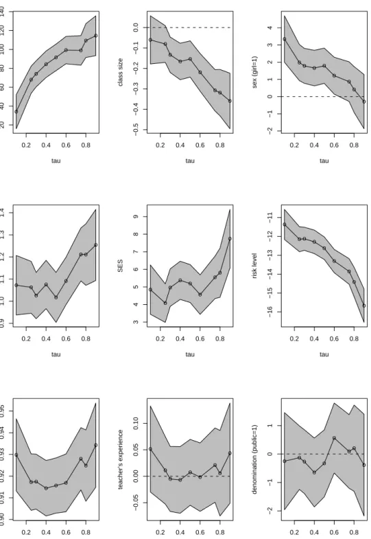
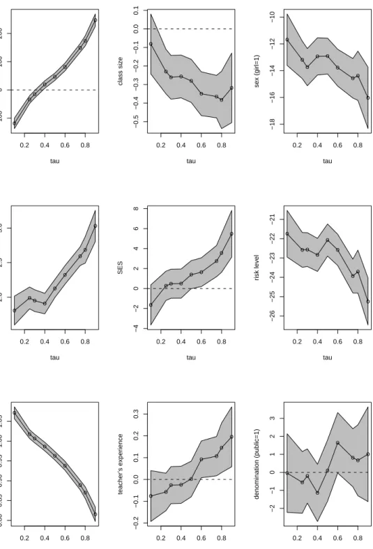
we briefly describe some preliminary quantile regression results based on treating class size as exogonous. These results are illustrated in Figures 6.2 and 6.3 for language and math performance, respectively. Considering the class size effect first. The plots suggest that class size effects are roughly similar for math and language performance: both are significant, both are downward sloping, indicating that while class size re-ductions are beneficial to all students they are more beneficial to better students conditional on the other covariates. The plots also suggest that peer effects are quite important especially for math, although considerable caution is required in the inter-pretation of these effects. Individual student characteristics are also quite interesting. Girls appear to be clearly disadvantaged in math, but exhibit a modest advantage in language. The “at risk” variable has a large impact, suggesting that students’ attitude and behavior towards school work is crucial for their scholastic performance, although again, exogoneity may be controversial. As expected, family background plays an important role in students’ academic performance, especially in language. Socio-economic status has a significantly positive effect across all quantiles of students achievement distribution and the effect increases as we move to higher quantiles of student achievement. IQ has the expected positive effect on students achievement with the magnitude of this effect larger on the math scores than on the language scores. Interestingly, more experienced teachers have no significant impact on lan-guage performance, but do seem to have a desirable effect on the upper quantiles of math performance. A public versus parochial school effect on student attainment is not distinguishable across the quantiles considered.
We now turn to the estimation of the class size effect in our structural framework. A concise visual summary of the structural estimates of the class size effect on language and math scores is provided in Figures 6.4 and 6.5 respectively. In the left panel we depict the conventional two stage least squares estimate of the mean shift effect of
class size viewed as a constant function of τ1 and τ2. In the middle panel we show
0.2 0.4 0.6 0.8 20 40 60 80 100 120 140 tau intercept o oo o o o o o o 0.2 0.4 0.6 0.8 −0.5 −0.4 −0.3 −0.2 −0.1 0.0 tau class size o o o o o o o o o 0.2 0.4 0.6 0.8 −2 −1 0 1 2 3 4 tau sex (girl=1) o oo o o o o o o 0.2 0.4 0.6 0.8 0.9 1.0 1.1 1.2 1.3 1.4 tau IQ o o o o o o o o o 0.2 0.4 0.6 0.8 3 4 5 6 7 8 9 tau SES o o o o o o oo o 0.2 0.4 0.6 0.8 −16 −15 −14 −13 −12 −11 tau risk level o o o o o o o o o 0.2 0.4 0.6 0.8 0.90 0.91 0.92 0.93 0.94 0.95 tau peer effects o o o o o o o o o 0.2 0.4 0.6 0.8 −0.05 0.00 0.05 0.10 tau teacher’s experience o o o o o o o o o 0.2 0.4 0.6 0.8 −2 −1 0 1 tau denomination (public=1) o oo o o o oo o
Figure 6.2. Quantile Regression Covariate Effects for Language Per-formance: Class Size Treated as Exogenous.
0.2 0.4 0.6 0.8 −100 0 100 200 tau intercept o oo o o o o o o 0.2 0.4 0.6 0.8 −0.5 −0.4 −0.3 −0.2 −0.1 0.0 0.1 tau class size o o o o o o o o o 0.2 0.4 0.6 0.8 −18 −16 −14 −12 −10 tau sex (girl=1) o o o o o o o o o 0.2 0.4 0.6 0.8 2.0 2.5 3.0 tau IQ o o o o o o oo o 0.2 0.4 0.6 0.8 −4 −2 0 2 4 6 8 tau SES o o o o o o o o o 0.2 0.4 0.6 0.8 −26 −25 −24 −23 −22 −21 tau risk level o o o o o o oo o 0.2 0.4 0.6 0.8 0.80 0.85 0.90 0.95 1.00 1.05 tau peer effects o o o o o o o o o 0.2 0.4 0.6 0.8 −0.2 −0.1 0.0 0.1 0.2 0.3 tau teacher’s experience o o o o o o o o o 0.2 0.4 0.6 0.8 −2 −1 0 1 2 3 tau denomination (public=1) o oo o o o o o o
Figure 6.3. Quantile Regression Covariate Effects for Math Perfor-mance: Class Size Treated as Exogenous.
0.2 0.4 0.6 0.8 tau1 0.2 0.4 0.6 0.8 tau2 -1.5 -1 -0.5 0 0.5 1 1.5 2 delta
Mean Treatment Effect
0.2 0.4 0.6 0.8 tau1 0.2 0.4 0.6 0.8 tau2 -1.5 -1 -0.5 0 0.5 1 1.5 2 delta(tau1)
Mean Quantile Treatment Effect
0.2 0.4 0.6 0.8 tau1 0.2 0.4 0.6 0.8 tau2 -1.5 -1 -0.5 0 0.5 1 1.5 2 delta(tau1, tau2)
Quantile Treatment Effect
Figure 6.4. Structural Class Size Effects for Language: τ1-students
achievement, τ2-class size.
0.2 0.4 0.6 0.8 tau1 0.2 0.4 0.6 0.8 tau2 -1 -0.5 0 0.5 1 delta
Mean Treatment Effect
0.2 0.4 0.6 0.8 tau1 0.2 0.4 0.6 0.8 tau2 -1 -0.5 0 0.5 1 delta(tau1)
Mean Quantile Treatment Effect
0.2 0.4 0.6 0.8 tau1 0.2 0.4 0.6 0.8 tau2 -1 -0.5 0 0.5 1 delta(tau1, tau2)
Quantile Treatment Effect
Figure 6.5. Structural Class Size Effects for Math: τ1-students
achievement, τ2-class size.
the τ2 effect from the weighted average derivative estimate of the ˆδ(τ1, τ2) estimate of
the structural class size effect. In the right panel we present ˆδ(τ1, τ2).
The two stage least squares estimate of the class size effect is -0.07 with a standard error of 0.20, a finding consistent with many other unsuccessful attempts to discern a significant effect of class size. However, our estimates of the mean quantile treatment effect of class size in the middle panel reveals a somewhat more nuanced view. Both math and language plots show a positive effect of around 0.7 at low quantiles and
0.2 0.4 0.6 0.8 −2 −1 0 1 2 WAD o o o o o o o o o 0.2 0.4 0.6 0.8 −2 −1 0 1 2 CV o o o o o o o o o 0.2 0.4 0.6 0.8 −2 −1 0 1 2 o o o o o o o o o 0.2 0.4 0.6 0.8 −2 −1 0 1 2 o o o o o o o o o 0.2 0.4 0.6 0.8 −2 −1 0 1 2 o o o o o o o o o 0.2 0.4 0.6 0.8 −2 −1 0 1 2 o o o o o o o o o 0.2 0.4 0.6 0.8 −2 −1 0 1 2 o o o o o o o o o 0.2 0.4 0.6 0.8 −2 −1 0 1 2 o o o o o o o o o 0.2 0.4 0.6 0.8 −2 −1 0 1 2 o o o o o o o o o 0.2 0.4 0.6 0.8 −2 −1 0 1 2 o o o o o o o o o
Figure 6.6. Structural Class Size Effect on Language Scores: The figure presents both the weighted average derivative (WAD) and control variate (CV) estimates of the structural class size effect on language performance. Five quantiles of the class size distribution are presented
for each estimator in descending order from the top of the plot τ2 ∈
{0.10,0.25,0.50,0.75,0.90}.
falling gradually to about -0.5 at the upper quantiles, suggesting that poorer students benefit from larger classes, while better students do better in smaller classes. Further disaggregating, the plots in the right panel indicate dispersion in the class size effect
0.2 0.4 0.6 0.8 −2 −1 0 1 2 WAD o o o o o o o o o 0.2 0.4 0.6 0.8 −2 −1 0 1 2 CV o o o o o o o o o 0.2 0.4 0.6 0.8 −2 −1 0 1 2 o o o o o o o o o 0.2 0.4 0.6 0.8 −2 −1 0 1 2 o o o o o o o o o 0.2 0.4 0.6 0.8 −2 −1 0 1 2 o o o o o o o o o 0.2 0.4 0.6 0.8 −2 −1 0 1 2 o o o o o o o o o 0.2 0.4 0.6 0.8 −2 −1 0 1 2 o o o o o o o o o 0.2 0.4 0.6 0.8 −2 −1 0 1 2 o o o o o o o o o 0.2 0.4 0.6 0.8 −2 −1 0 1 2 o o o o o o o o o 0.2 0.4 0.6 0.8 −2 −1 0 1 2 o o o o o o o o o
Figure 6.7. Structural Class Size Effect on Math Scores: The fig-ure presents both the weighted average derivative (WAD) and control variate (CV) estimates of the structural class size effect on mathemat-ics performance. Five quantiles of the class size distribution are pre-sented for each estimator in descending order from the top of the plot
τ2 ∈ {0.10,0.25,0.50,0.75,0.90}.
at the lower quantiles of test scores, and negative effects at the upper quantiles. In such circumstances it is not surprising that averaging over both quantile dimensions yields a result that is statistically negligible.
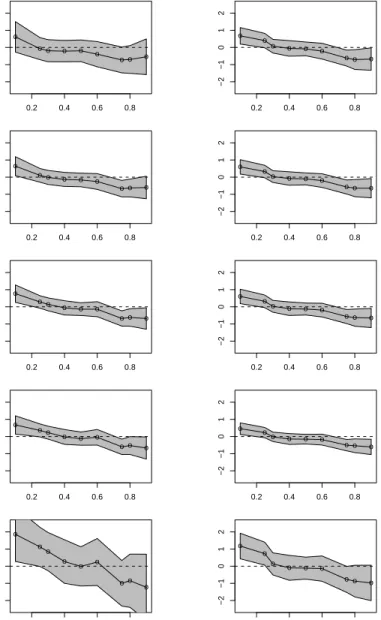
To examine the structural estimates more closely we plot in Figures 6.6 and 6.7 cross-sectional slices of the foregoing perspective plots. Superimposed on these plots is a .90 (pointwise) confidence band. To contrast the weighted average derivative approach and the control variate method we illustrate both estimates in Figure 6.6 for language performance and in Figure 6.7 for math. The similarity of the WAD and CV estimates provides some support for the model specification. We summarize our findings briefly as follows:
• The class size effect on language scores:
– For weaker students the plots indicate that bigger classes are better.
– For near median students class size effects are not significant.
– For better students smaller classes appear marginally better.
• The class size effect on math scores:
– For weaker students smaller classes are better
– For the average and good students the class size effect is not significant.
Our finding that class size has an insignificant influence on median performance in language and math is quite consistent with previous literature indicating similarly insignificant conditional mean effects. However, especially in the case of language performance, we find that one should interpret findings of insignificant mean effects with considerable caution since it appears that they arise from averaging significant benefits from reductions in class size for good students and significant benefits from increases in class size for poorer students.
We would again stress the point that changes in class sizes per se cannot produce
academic gains, but in combination with other instructional practices and institua-tional arrangements such changes may have benefits. By providing a more nuanced view of the apparently heterogeneous effects of class size, structural methods based on quantile regression may be able to constructively contribute to the policy debate on these important issues.
Appendix A. proofs
Lemma 1. Let Y andZ be N×K matrices of rank K and X be a N×L matrix of rank L. Ifβˆ1= (Z>MXZ)−1Z>MXY, with MX =I−X(X>X)−1X>, then (A.1) 1 βˆ1−1 Y>MXY Y>MXZ Z>MXY Z>MXZ −1 = 0 βˆ1−1(Z>MXZ)−1 .
Proof: Define ˜Y =MXY and ˜Z =MXZ, we have: ˜ Y>Y˜ Y˜>Z˜ ˜ Z>Y˜ Z˜>Z˜ −1 = ( ˜Y>MZ˜Y˜)−1 F F> ( ˜Z>MY˜Z˜)−1 , (A.2) where F satisfies ( ˜Y>MZ˜Y˜)−1Y˜>Z˜+FZ˜>Z˜= 0, (A.3) or, ( ˜Z>MY˜Z˜)−1Z˜>Z˜+F>Y˜>Z˜=I. (A.4)