Auto-Balancing Two Wheeled Inverted Pendulum Robot

Vol. X, No. X, 2014

163 Available online at www.ijiere.com

International Journal of Innovative and Emerging

Research in Engineering

e-ISSN: 2394 – 3343 p-ISSN: 2394 – 5494

Auto-Balancing Two Wheeled Inverted Pendulum Robot

Om J. Sawant

_{, Shubhada Deshpande}

_{, Ashish Lele}

_{, Sejal Jamsandekar}

_{and Rohit Patil}

a_{Pursuing B.E., Department of Electronics, PVPPCOE, Sion, Mumbai, India} b_{Professor, Department of Electronics, PVPPCOE, Sion, Mumbai, India}

ABSTRACT:

The inverted pendulum platform is an example of classic unstable control system [4]_{. Although it is a fairly tested}

and documented concept, it draws attention of many researchers due to its application in auto balancing two-wheeled robots. Auto balancing two two-wheeled robot is characterized by its ability to balance on coaxial two wheels and to spin on a smaller base space. This provides with enormous advantage to maneuver in small and tidy work spaces, which is a drawback issue in case of conventional four wheeled robots. The work presented here focuses on implementation of inverted pendulum auto balancing robot by means of a stable control system. This paper enlightens the use of Kalman filter and PID controller algorithms to achieve the desired stability of the inverted pendulum system by discrete digital algorithmic approach.

Keywords: Inverted Pendulum, Control system, Kalman Filter, Sensor fusion, PID controller.

I. INTRODUCTION

A. Problem statement:

Auto balancing two wheeled robot will come out as an effective and unconventional way of maneuverability which is needed in many robotic applications. However, inverted pendulum platform is an unstable control system and hence faces stability issues [3]_{. Various control system models are proposed to stabilize the IP system.}

The output of inertial sensors used is noisy and filtering of raw output of sensors is required before it is fed to the microcontroller for reliable performance. Also, due to the nonlinear behavior of control system, we face linear filtering problem of discrete data.

Another major problem can be data sampling rate and computation time required by microcontroller to run control algorithm. Excessive computation delay leads to more time for correction of the tilt angle of inverted pendulum and leaves the system out of vertical equilibrium position.

As compared to conventional robots, it is observed that the power required for driving DC motors to maintain equilibrium position is very high in case of auto balancing robots. Taking into consideration the higher design complexity and lower design flexibility, the cost of some components can lead to the question of cost effectiveness of entire project.

B. Problem solving:

The self-balancing robot structure is modeled on inverted pendulum problem. The goal of presented work will be to investigate the use of digital control algorithm implemented on a microcontroller as solution to above problem. The digital control algorithm used is Proportional-Integral-Derivative controller, which works to minimize the error and attain the vertical equilibrium position of the inverted pendulum to make the system stable.

The sensors used are inertial sensors viz. accelerometer and gyroscope to give information about tilt angle of the inverted pendulum. To filter the noisy outputs of these sensors, the use of Kalman Filter algorithm is vital feature of this project. Kalman filter algorithm is estimating in nature and can also be used for fusing the outputs of both the sensors to give reliable tilt angle information.

Over the period of time microcontrollers are providing versatile, quicker, cheaper and reliable options. This project will be built around a powerful but cost effective development board having ARM Cortex M0+ core microcontroller architecture. The Kalman Filter algorithm and PID controller logic will be implemented on the above said microcontroller. This provides the required cost effectiveness along with low power consumption.

Vol. X, No. X, 2014

164

II. PHYSICAL AND MATHEMATICAL MODEL

As given in Joe: A mobile, inverted pendulum [2]_{,considering the robot with its three degrees of freedom, it is able to}

rotate about its z axis (pitch). A movement described by angle θP and corresponding angular velocity ωP. The linear motion

of robot is given with XRM and velocity VRM. Additionally, the vehicle can rotate around its vertical axis (yaw) with the

associated angle δ and angular velocity δ’.

Various disturbances are the forces acting on, the center of gravity (CG) of the vehicle, fdP, the center of the left wheel,

fdRL, the center of the right wheel, fdRR.

The vehicle is controlled by applying a torque CL and CR to the corresponding wheels.

In order to successfully control the system, the state-space variables have to be quantified. XRM, VRM, δ and δ’ can be

easily determined with the help of encoders mounted on the two wheels (provided θP and ωP are known).

Figure 1. Free-body diagram of robot [2]

For developing an efficient control system for the robot, its mathematical model has to be designed. The following variables have been chosen to describe mathematical model of robot.

JRL, JRR —moment of inertia of the rotating masses with respect to the axis;

MRL, MRR —mass of the rotating masses connected to the left and right wheels;

JPθ —moment of inertia of the chassis with respect to the axis;

JPδ —moment of inertia of the chassis with respect to the axis;

MP —mass of the chassis;

R —radius of the wheels;

D —lateral distance between the contact patches of the wheels; L —distance between the axis and the CG of the chassis.

The following set of equations of motion can be obtained from free body diagram: For wheels

 x”RLMRL= fdRL – HL + HTL  y”RLMRL = VTL – MRLg - VL  θ”

RLJRL = CL – HTLR For the Chassis

 x”PMP = fdP + HR + HL  y”PMP = VR + VL – MPg + FCθ  θ”

PJPθ = (VR + VL).L.sinθP – (HR + HL).L.cosθP – (CL + CR)  δ”_{JPδ = (H}

L – HR)D/2

Where HL, HR, HTL, HTR, VL, VR, VTL, VTR represent the reaction forces acting on different parts of free body.

Modifying equations 1 to 7 and then linearizing the result around the operating point (XRM = 0; θP = 0 and δ = 0) the

Vol. X, No. X, 2014

165 Figure 2. State-space representation

This state-space representation can be used for designing control system.

III. IMPLEMENTATION

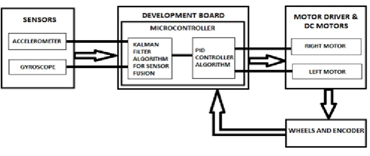
This part of the paper proposes the implementation of the Auto-Balancing Two Wheeled Robot. The task of balancing inverted pendulum is very complex if we try to derive a single Transfer Function equation considering the project as a single control system. This may be achieved theoretically but practical implementation will not be as per expectation. Due to the large number of physical unknown parameters governing the state of control system, the single transfer function approach would be impractical to achieve stability in real time implementation of project. To avoid this complexity we will break the control system into basic blocks. Every block dealing with the fixed number of variables and serving its successive block. The blocks used for implementation of project are specified with block diagram.

A. Block Diagram:

Figure 3. Block diagram

B. Sensors:

Sensors used in this project include accelerometer and gyroscope. These are inertial sensors used to provide tilt angle and rate of fall of angle i.e. angular rate. The data from the sensors will give sense of angular displacement of the inverted pendulum from its vertical zero equilibrium position. As the primary goal of this project is to maintain zero degree vertical angle of inverted pendulum, the measurement of instantaneous angle of structure becomes very important.

The digital rate gyroscope gives information about instantaneous rate of change of angle. The rest state offset value of gyroscope must be measured and the device should be calibrated. But it is observed that gyroscope produces a significant drift when operating. This drift may be due to temperature or inherent characteristics of gyroscope itself.

On the other hand, accelerometer gives absolute measure of tilt angle. But it is observed that the output signal is often corrupted with significant amount of noise.

Generalized sensor equations: For Gyroscope

 ADCresol = Vcc / 2nbit

 GYROresol = (ADCresol / GYROsensitivity)  GYROoffset = (Vstatic . 2nbit) / Vcc

 ANGULAR_RATE = (ADCresol – GYROoffset) . GYROresol For Accelerometer

Vol. X, No. X, 2014

166  ACCLresol = ( 1g . ADCresol ) / 1000mV

 ACCLoffset = (Voffset . 2nbit) / Vcc

 Ax = (ADCresol – ACCLoffset) . ACCLresol  Pitch = sin-1_(A

x/1g)

From above discussion about sensors one can state that the use of any of the sensor alone to achieve tilt angle information is not sufficient in order to balance the robot. Because the information provided by sensors is insufficient and unreliable. To get rid of this problem, use of signal level sensor fusion becomes mandatory. Sensor fusion refers to combining output signals of sensors to give an improved and reliable signal. Kalman Filter is used for the same, which uses accelerometer signal to eliminate the drift problem in gyroscope output and gives accurate estimate of tilt angle and its derivative term.

C. Kalman Filter:

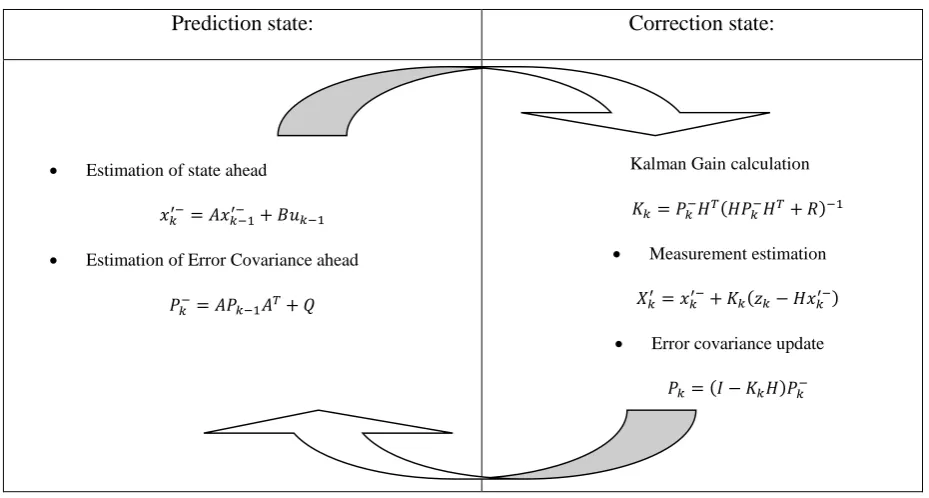
Kalman filter is basically recursive digital algorithm which can be used for estimation of state of any process [5] [6]_{. Due}

to its state estimating nature it provides reliable state estimate. Kalman filter also has a feature of minimizing mean square error. Hence it can be applied to control systems operating in noisy environment. Kalman filter processes the output signals from sensors and minimizes square error. Then this noise free signal can be fed to control system for reliable output response.

Kalman filter estimates the state of discrete time controlled process given in linear stochastic difference equation form: xk = Axk – 1 + Buk – 1 + wk – 1

Measurement: zk = Hxk + vk

Random variables vk and wk are measurement noise and process noise respectively. They have normal probability

distribution as: p(w) = N(0, Q) p(v) = N(0, R)

Where Q is process noise covariance matrix and R is measurement noise covariance matrix. Matrices A and H are state matrices relating state of next time step and measurement state respectively. Matrix B is related to control input u of process x.

Kalman filter equations can be distinguished in two states, predictions state and correction state. The prediction state is nothing but time updating phenomenon. In prediction state, considering current time state and error covariance estimate, new state is estimated. The correction state produces a feedback to generate estimate of next measurement.

Table 1. Kalman filter equations

Prediction state:

Correction state:

 Estimation of state ahead

𝑥𝑘′−= 𝐴𝑥𝑘−1′− + 𝐵𝑢𝑘−1

 Estimation of Error Covariance ahead

𝑃𝑘−= 𝐴𝑃𝑘−1𝐴𝑇+ 𝑄

Kalman Gain calculation

𝐾𝑘= 𝑃𝑘−𝐻𝑇(𝐻𝑃𝑘−𝐻𝑇+ 𝑅)−1

 Measurement estimation

𝑋_𝑘′ _{= 𝑥}

𝑘′−+ 𝐾𝑘(𝑧𝑘− 𝐻𝑥𝑘′−)

 Error covariance update

𝑃𝑘= (𝐼 − 𝐾𝑘𝐻)𝑃𝑘−

D. PID controller:

Vol. X, No. X, 2014

167 change of the signal. It uses closed loop control system approach. The algorithm is best suited when the process under control is modeled as a linear system.

The PID controller consists of proportional, integral, and derivative terms. The KP, KI, and KD are referred as the proportional, integral, and derivative constants. The terms of the PID controller are summed up to create a controller output signal. Each term performs a different task in the control process. The controller terms also have different effects on the system output response.

It is also referred as a negative feedback system. The basic idea of a negative feedback system is that it measures the process output y using a sensor. The measured process output gets subtracted from the reference set-point value to produce an error. The error is then fed into the PID controller, where the error gets processed in three ways. The error will be used on the PID controller to execute the proportional term, integral term reduces the steady state errors, and the derivative term handles overshoots. After the PID algorithm processes the error, the controller produces a control signal u. The PID control signal u will try to drive the process to the desired reference set-point value. In the case of the two wheel robot, the desired set-point value is the zero degree vertical position.

Equations given below represents PID controller in continuous time domain. TD and TI are time constants for derivative

and integral term respectively.

 𝑒𝑟𝑟𝑜𝑟 = 𝑟𝑒𝑓 − 𝑦  𝑢(𝑡) = 𝐾𝑝(𝑒𝑟𝑟𝑜𝑟(𝑡) + 1 𝑇𝐼∫ 𝑒𝑟𝑟𝑜𝑟(𝑡)𝑑𝑡 + 𝑇𝐷 𝑑𝑒𝑟𝑟𝑜𝑟(𝑑𝑡) 𝑑𝑡 1 0 ) Where, 𝐾𝐼= 𝐾_𝑃 𝑇𝐼, 𝐾𝐷 = 𝐾𝑃𝑇𝐷  𝑢(𝑡) = 𝐾𝑝𝑒𝑟𝑟𝑜𝑟(𝑡) + 𝐾𝐼∫ 𝑒𝑟𝑟𝑜𝑟(𝑡)𝑑𝑡 + 𝐾𝐷 𝑑𝑒𝑟𝑟𝑜𝑟(𝑑𝑡) 𝑑𝑡 1 0

Discrete PID controller algorithm:

As we are implementing PID algorithm on a micro-controller, it is necessary to design the PID equations in discrete time domain. Trying to develop PID software algorithm that follows discrete time domain notations is practically not possible. Only approach to achieve PID controller algorithm in discrete time domain notations is by approximation of terms of PID controller equations in continuous time domain given above. The discrete representation of the controller makes it easier to implement the PID algorithm on a micro-controller

The equations given below represents PID controller in discrete form:  ∫ 𝑒𝑟𝑟𝑜𝑟(𝑡)𝑑𝑡 ≈ 𝑇𝑆∑𝑘=1𝑒𝑟𝑟𝑜𝑟(𝑘)

1 0  𝑑𝑒𝑟𝑟𝑜𝑟(𝑡) 𝑑𝑡 ≈ 𝑒𝑟𝑟𝑜𝑟(𝑘)−𝑒𝑟𝑟𝑜𝑟(𝑘−1) 𝑇𝑆  𝑢(𝑘) = 𝐾𝑝(𝑒𝑟𝑟𝑜𝑟(𝑘) + 𝑇𝑆 𝑇𝐼∑ 𝑒𝑟𝑟𝑜𝑟(𝑘) + 𝑇𝐷

𝑇𝑆(𝑒𝑟𝑟𝑜𝑟(𝑘) − 𝑒𝑟𝑟𝑜𝑟(𝑘 − 1))

𝑘=1 ) 𝑊ℎ𝑒𝑟𝑒, 𝐾𝐼 = 𝐾𝑃 𝑇𝑆 𝑇𝐼 𝐾𝐷 = 𝐾𝑃 𝑇𝐷 𝑇𝑆



E. DC MOTORS AND MOTOR DRIVER:

The selection of motors is an important aspect in designing the Auto Balancing Robot System. The motors should have adequate torque rating and also should have appropriate RPM value for proper functioning of the self- balancing mechanism. Also, the motors should be of moderate voltage and current requirement to keep the power supply less bulky and make the driver circuit less complex.

To suit the requirements of the project, two DC motors of the following specifications have been proposed:  Maximum Supply Voltage: 9V DC

 Torque Rating: 2kg/cm  RPM at no load: 100

Vol. X, No. X, 2014

168 The motor driver circuit L298N is being used in this project. The circuit is a high voltage, high current dual full bridge driver.

The features of the driver module are as follows [7]_:

. OPERATING SUPPLY VOLTAGE UP TO 46 V . TOTAL DC CURRENT UP TO 4 A

. LOW SATURATION VOLTAGE . OVERTEMPERATURE PROTECTION

. LOGICAL "0" INPUT VOLTAGE UP TO 1.5 V (HIGH NOISE IMMUNITY)

F. Encoder:

Encoder is an important block in the closed loop control system. It consists of a tachometer which measures the frequency of rotation of wheels and converts the frequency into corresponding voltage signal. Hence encoder is nothing but frequency to voltage converter. Voltage signal produced by encoder is fed as negative feedback to the PID controller. In this way encoder completes the negative feedback in PID controller. By comparing the signal given by encoder with the set-point condition, error will be calculated and then PID controller processes the error to minimize it.

IV.CONCLUSION

It can be concluded that, after implementation of this project, the stability of Auto-Balancing Two Wheeled Inverted Pendulum Robot can be achieved with improved response time. We have considered the system of robot as a classical control system and proposed the algorithmic approach to stabilize the system. Through this paper we are implementing Kalman filter algorithm and PID controller digital control algorithm on a micro-controller, which gives cost-effective option for solving Inverted Pendulum control system problem with reduced oscillations and improved stability. Our emphasis is on achieving zero degree vertical equilibrium of robot body when it is in rest or when it is in a straight line motion, in shortest possible time. Further study can be done on achieving the stability of robot while rotating about its vertical axis.

ACKNOWLEDGMENT

This work is supported by Department of Electronics Engineering, Padmabhushan Vasantdada Patil Pratishthan’s College of Engineering, Sion, Mumbai

.

REFERENCES

[1] Spong M.W., Hutchinson S., Vidyasagar M.: Robot modeling and control, Wiley, 2006

[2] F. Grasser, A. D’Arrigo, S. Colombi, and A. Rufer, “Joe: A mobile, inverted pendulum”, IEEE Trans. Ind. Electron., vol. 49, no. 1, pp.107–114, Feb. 2002

[3] Li Chaoquan, Gao Xueshan, Li Kejie, “Smooth Control the Coaxial Self-Balance Robot under Impact Disturbances”, International Journal of Advanced Robotic Systems,ISSN 1729-8806, pp 59-67 Vol. 8, No. 2. (2011)

[4] Kent H. Lundberg, James K. Roberge, “Classical Dual-Inverted-Pendulum Control,” THE 2003 IEEE CONFERENCE ON DECISION AND CONTROL, 2003

[5] R. E. Kalman, “A New Approach to Linear Filtering and Prediction Problems,” Transaction of the ASME— Journal of Basic Engineering, pp. 35-45 (March 1960).