A Statistical Perspective on Randomized Sketching
for Ordinary Least-Squares
Garvesh Raskutti [email protected]
Department of Statistics
University of Wisconsin–Madison Madison, WI 53706, USA
Michael W. Mahoney [email protected]
International Computer Science Institute and Department of Statistics University of California at Berkeley
Berkeley, CA 94720, USA
Editor:Mehryar Mohri
Abstract
We consider statistical as well as algorithmic aspects of solving large-scale least-squares (LS) problems using randomized sketching algorithms. For a LS problem with input data (X, Y) ∈ Rn×p×
Rn, sketching algorithms use a “sketching matrix,” S ∈ Rr×n, where r n. Then, rather than solving the LS problem using the full data (X, Y), sketching algorithms solve the LS problem using only the “sketched data” (SX, SY). Prior work has typically adopted analgorithmic perspective, in that it has made no statistical assumptions on the inputX andY, and instead it has been assumed that the data (X, Y) are fixed and worst-case (WC). Prior results show that, when using sketching matrices such as random projections and leverage-score sampling algorithms, with p.rn, the WC error is the same as solving the original problem, up to a small constant. From astatistical perspective, we typically consider the mean-squared error performance of randomized sketching algo-rithms, when data (X, Y) are generated according to a statistical linear modelY =Xβ+, whereis a noise process. In this paper, we provide a rigorous comparison of both perspec-tives leading to insights on how they differ. To do this, we first develop a framework for assessing, in a unified manner, algorithmic and statistical aspects of randomized sketching methods. We then consider the statistical prediction efficiency (PE) and the statistical residual efficiency (RE) of the sketched LS estimator; and we use our framework to provide upper bounds for several types of random projection and random sampling sketching algo-rithms. Among other results, we show that the RE can be upper bounded whenp.rn
while the PE typically requires the sample sizerto be substantially larger. Lower bounds developed in subsequent results show that our upper bounds on PE can not be improved.1
Keywords: algorithmic leveraging, randomized linear algebra, sketching, random pro-jection, statistical leverage, statistical efficiency
1. Introduction
Recent work in large-scale data analysis has focused on developing so-called sketching al-gorithms: given a data set and an objective function of interest, construct a small “sketch”
of the full data set, e.g., by using random sampling or random projection methods, and use that sketch as a surrogate to perform computations of interest for the full data set (see Ma-honey (2011) for a review). Most effort in this area has adopted analgorithmic perspective, whereby one shows that, when the sketches are constructed appropriately, one can obtain answers that are approximately as good as the exact answer for the input data at hand, in less time than would be required to compute an exact answer for the data at hand. In statistics, however, one is often more interested in how well a procedure performs relative to an hypothesized model than how well it performs on the particular data set at hand. Thus an important to question to consider is whether the insights from the algorithmic perspective of sketching carry over to the statistical setting.
Thus, in this paper, we develop a unified approach that considers both the statistical
perspective as well as algorithmic perspective on recently-developed randomized sketching
algorithms, and we provide bounds on two statistical objectives for several types of random projection and random sampling sketching algorithms.
1.1 Overview of the Problem
The problem we consider in this paper is the ordinary least-squares (LS or OLS) problem: given as input a matrixX ∈Rn×pof observed features or covariates and a vectorY ∈
Rnof
observed responses, return as output a vector βOLS that solves the following optimization
problem:
βOLS = arg min β∈Rp
kY −Xβk22. (1)
We will assume that n and p are both very large, with n p, and for simplicity we will assume rank(X) =p, e.g., to ensure a unique full-dimensional solution. The OLS solution,
βOLS = (XTX)−1XTY, has a number of well-known desirable statistical properties
(Chat-terjee and Hadi, 1988); and it is also well-known that the running time or computational complexity for this problem isO(np2) (Golub and Loan, 1996).2 For many modern applica-tions, however,nmay be on the order of 106−109 and pmay be on the order of 103−104, and thus computing the exact LS solution with traditionalO(np2) methods can be compu-tationally challenging. This, coupled with the observation that approximate answers often suffice for downstream applications, has led to a large body of work on developing fast approximation algorithms to the LS problem (Mahoney, 2011).
One very popular approach to reducing computation is to perform LS on a carefully-constructed “sketch” of the full data set. That is, rather than computing a LS estimator from Problem (1) from the full data (X, Y), generate “sketched data” (SX, SY) where
S ∈Rr×n, withrn, is a “sketching matrix,” and then compute a LS estimator from the
following sketched problem:
βS ∈arg min β∈Rp
kSY −SXβk2
2. (2)
2. That is,O(np2) time suffices to compute the LS solution from Problem (1) for arbitrary or worst-case
Once the sketching operation has been performed, the additional computational complexity of βS is O(rp2), i.e., simply call a traditional LS solver on the sketched problem. Thus,
when using a sketching algorithm, two criteria are important: first, ensure the accuracy of the sketched LS estimator is comparable to, e.g., not much worse, than the performance of the original LS estimator; and second, ensure that computing and applying the sketching matrixS is not too computationally intensive, e.g., that is faster than solving the original problem exactly.
1.2 Prior Results
Random sampling and random projections provide two approaches to construct sketching matrices S that satisfy both of these criteria and that have received attention recently in the computer science community. Very loosely speaking, a random projection matrixS is a dense matrix,3 where each entry is a mean-zero bounded-variance Gaussian or Rademacher random variable, although other constructions based on randomized Hadamard transfor-mations are also of interest; and a random sampling matrix S is a very sparse matrix that has exactly 1 non-zero entry (which typically equals one multiplied by a rescaling factor) in each row, where that one non-zero can be chosen uniformly, non-uniformly based on hypotheses about the data, or non-uniformly based on empirical statistics of the data such as the leverage scores of the matrix X. In particular, note that a sketch constructed from anr×nrandom projection matrixS consists ofr linear combinations of most or all of the rows of (X, Y), and a sketch constructed from a random sampling matrix S consists of r
typically-rescaled rows of (X, Y). Random projection algorithms have received a great deal of attention more generally, largely due to their connections with the Johnson-Lindenstrauss lemma (Johnson and Lindenstrauss, 1984) and its extensions; and random sampling algo-rithms have received a great deal of attention, largely due to their applications in large-scale data analysis applications (Mahoney and Drineas, 2009). A detailed overview of random projection and random sampling algorithms for matrix problems may be found in the recent monograph of Mahoney (2011). Here, we briefly summarize the most relevant aspects of the theory.
In terms of running time guarantees, the running time bottleneck for random projec-tion algorithms for the LS problem is the applicaprojec-tion of the projecprojec-tion to the input data, i.e., actually performing the matrix-matrix multiplication to implement the projection and compute the sketch. By using fast Hadamard-based random projections, however, Drineas et al. (2011) developed a random projection algorithm that runs on arbitrary or worst-case input ino(np2) time. (See Drineas et al. (2011) for a precise statement of the running time.) As for random sampling, it is trivial to implement uniform random sampling, but it is very easy to show examples of input data on which uniform sampling performs very poorly. On the other hand, Drineas et al. (2006b, 2012) have shown that if the random sampling is performed with respect to nonuniform importance sampling probabilities that depend on
the empirical statistical leverage scores of the input matrix X, i.e., the diagonal entries of
the hat matrix H =X(XTX)−1XT, then one obtains a random sampling algorithm that
achieves much better results for arbitrary or worst-case input.
Leverage scores have a long history in robust statistics and experimental design. In the robust statistics community, samples with high leverage scores are typically flagged as potential outliers (see, e.g., Chatterjee and Hadi (2006, 1988); Hampel et al. (1986); Hoaglin and Welsch (1978); Huber and Ronchetti (1981)). In the experimental design community, samples with high leverage have been shown to improve overall efficiency, provided that the underlying statistical model is accurate (see, e.g., Royall (1970); Zavlavsky et al. (2008)). This should be contrasted with their use in theoretical computer science. From the al-gorithmic perspective of worst-case analysis, that was adopted by Drineas et al. (2011) and Drineas et al. (2012), samples with high leverage tend to contain the most important information for subsampling/sketching, and thus it is beneficial for worst-case analysis to bias the random sample to include samples with large statistical leverage scores or to rotate to a random basis where the leverage scores are approximately uniformized.
The running-time bottleneck for this leverage-based random sampling algorithm is the computation of the leverage scores of the input data; and the obvious well-known algorithm for this involvesO(np2) time to perform a QR decomposition to compute an orthogonal basis forX(Golub and Loan, 1996). By using fast Hadamard-based random projections, however, Drineas et al. (2012) showed that one can compute approximate QR decompositions and thus approximate leverage scores ino(np2) time, and (based on previous work (Drineas et al., 2006b)) this immediately implies a leverage-based random sampling algorithm that runs on arbitrary or worst-case input ino(np2) time (Drineas et al., 2012). Readers interested in the practical performance of these randomized algorithms should consult Bendenpik (Avron
et al., 2010) orLSRN(Meng et al., 2014).
In terms of accuracy guarantees, both Drineas et al. (2011) and Drineas et al. (2012) prove that their respective random projection and leverage-based random sampling LS sketching algorithms each achieve the following worst-case (WC) error guarantee: for any arbitrary (X, Y),
kY −XβSk22 ≤(1 +κ)kY −XβOLSk22, (3)
with high probability for some pre-specified error parameterκ∈(0,1).4 This 1 +κ relative-error guarantee5 is extremely strong, and it is applicable to arbitrary or worst-case input. That is, whereas in statistics one typically assumes a model, e.g., a standard linear model on Y,
Y =Xβ+, (4)
whereβ∈Rp is the true parameter and∈
Rnis a standardized noise vector, withE[] = 0
and E[T] = In×n, in Drineas et al. (2011) and Drineas et al. (2012) no statistical model
is assumed on X and Y, and thus the running time and quality-of-approximation bounds apply to any arbitrary (X, Y) input data.
1.3 Our Approach and Main Results
In this paper, we adopt a statistical perspective on these randomized sketching algorithms, and we address the following fundamental questions. First, under a standard linear model, e.g., as given in Eqn. (4), what properties of a sketching matrix S are sufficient to ensure
4. The quantitykβS−βOLSk22 is also bounded by Drineas et al. (2011) and Drineas et al. (2012).
5. The nonstandard parameterκis used here for the error parameter since is used below to refer to the
low statistical error, e.g., mean-squared, error? Second, how do existing random projec-tion algorithms and leverage-based random sampling algorithms perform by this statistical measure? Third, how does this relate to the properties of a sketching matrix S that are sufficient to ensure low worst-case error, e.g., of the form of Eqn. (3), as has been estab-lished previously in Drineas et al. (2011, 2012); Mahoney (2011)? We address these related questions in a number of steps.
In Section 2, we will present a framework for evaluating the algorithmic and statistical properties of randomized sketching methods in a unified manner; and we will show that providing worst-case error bounds of the form of Eqn. (3) and providing bounds on two related statistical objectives boil down to controlling different structural properties of how the sketching matrix S interacts with the left singular subspace of the design matrix. In particular, we will consider the oblique projection matrix, ΠUS = U(SU)†S, where (·)† denotes the Moore-Penrose pseudo-inverse of a matrix and U is the left singular matrix of
X. This framework will allow us to draw a comparison between the worst-case error and two related statistical efficiency criteria, the statistical prediction efficiency (PE) (which is based on the prediction error E[kX(βb−β)k22] and which is given in Eqn. (7) below) and
the statistical residual efficiency (RE) (which is based on residual error E[kY −Xβkb 22] and
which is given in Eqn. (8) below); and it will allow us to provide sufficient conditions that any sketching matrix S must satisfy in order to achieve performance guarantees for these two statistical objectives.
In Section 3, we will present our main theoretical results, which consist of bounds for these two statistical quantities for variants of random sampling and random projection sketching algorithms. In particular, we provide upper bounds on the PE and RE (as well as the worst-case WC) for four sketching schemes: (1) an approximate leverage-based random sampling algorithm, as is analyzed by Drineas et al. (2012); (2) a variant of leverage-based random sampling, where the random samples arenotre-scaled prior to their inclusion in the sketch, as is considered by Ma et al. (2014, 2015); (3) a vanilla random projection algorithm, where S is a random matrix containing i.i.d. Gaussian or Rademacher random variables, as is popular in statistics and scientific computing; and (4) a random projection algorithm, where S is a random Hadamard-based random projection, as analyzed in Boutsidis and Gittens (2013). For sketching schemes (1), (3), and (4), our upper bounds for each of the two measures of statistical efficiency are identical up to constants; and they show that the RE scales as 1 + pr, while the PE scales as nr. In particular, this means that it is possible to obtain good bounds for the RE when p . r n (in a manner similar to the sampling complexity of the WC bounds); but in order to obtain even near-constant bounds for PE, r must be at least of constant order compared to n. We then present a lower bound developed in subsequent work by Pilanci and Wainwright (2014) which shows that under general conditions onS, our upper bound of nr for PE can not be improved. For the sketching scheme (2), we show, on the other hand, that under the strong assumption that there arek“large” leverage scores and the remainingn−kare “small,” then the WC scales as 1 + pr, the RE scales as 1 + pkrn, and the PE scales as kr. That is, sharper bounds are possible for leverage-score sampling without re-scaling in the statistical setting, but much stronger assumptions are needed on the input data.
versus random projection methods. Our empirical results support our theoretical results, and they also show that forr larger than p but much closer top than n, projection-based methods tend to out-perform sampling-based methods, while forr significantly larger than
p, our leverage-based sampling methods perform slightly better. In Section 5, we will provide a brief discussion and conclusion and we provide proofs of our main results in the Appendix.
1.4 Additional Related Work
Very recently Ma et al. (2014) considered statistical aspects of leverage-based sampling algo-rithms (calledalgorithmic leveragingin Ma et al. (2014)). Assuming a standard linear model onY of the form of Eqn. (4), the authors developed first-order Taylor approximations to the statistical relative efficiency of different estimators computed with leverage-based sampling algorithms, and they verified the quality of those approximations with computations on real and synthetic data. Taken as a whole, their results suggest that, if one is interested in the statistical performance of these randomized sketching algorithms, then there are nontrivial trade-offs that are not taken into account by standard worst-case analysis. Their approach, however, does not immediately apply to random projections or other more general sketching matrices. Further, the realm of applicability of the first-order Taylor approximation was not precisely quantified, and they left open the question of structural characterizations of random sketching matrices that were sufficient to ensure good statistical properties on the sketched data. We address these issues in this paper.
After the appearance of the original technical report version of this paper (Raskutti and Mahoney, 2014), we were made aware of subsequent work by Pilanci and Wainwright (2014), who also consider a statistical perspective on sketching. Amongst other results, they develop a lower bound which confirms that using a single randomized sketching matrix S can not achieve a PE better than nr. This lower bound complements our upper bounds developed in this paper. Their main focus is to use this insight to develop an iterative sketching scheme which yields bounds on the PE when an r×nsketch is applied repeatedly.
2. General Framework and Structural Results
In this section, we develop a framework that allows us to view the algorithmic and statistical perspectives on LS problems from a common perspective. We then use this framework to show that existing worst-case bounds as well as our novel statistical bounds for the mean-squared errors can be expressed in terms of different structural conditions on how the sketching matrix S interacts with the data (X, Y).
2.1 A Statistical-Algorithmic Framework
Recall that we are given as input a data set, (X, Y)∈Rn×p×
Rn, and the objective function
of interest is the standard LS objective, as given in Eqn. (1). Since we are assuming, without loss of generality, that rank(X) =p, we have that
where (·)† denotes the Moore-Penrose pseudo-inverse of a matrix, and where the second equality follows since rank(X) =p.
To present our framework and objectives, let S ∈ Rr×n denote an arbitrary sketching
matrix. That is, although we will be most interested in sketches constructed from random sampling or random projection operations, for now we let S be any r×n matrix. Then, we are interested in analyzing the performance of objectives characterizing the quality of a “sketched” LS objective, as given in Eqn (2), where again we are interested in solutions of the form
βS= (SX)†SY. (6)
(We emphasize that this doesnotin general equal ((SX)TSX)−1(SX)TSY, since the inverse will not exist if the sketching process does not preserve rank.) Our goal here is to compare the performance of βS to βOLS. We will do so by considering three related performance
criteria, two of a statistical flavor, and one of a more algorithmic or worst-case flavor. From a statistical perspective, it is common to assume a standard linear model on Y,
Y =Xβ+,
where we remind the reader thatβ∈Rp is the true parameter and∈Rnis a standardized
noise vector, with E[] = 0 and E[T] = In×n. From this statistical perspective, we will
consider the following two criteria.
• The first statistical criterion we consider is theprediction efficiency (PE), defined as follows:
CP E(S) = E
[kX(β−βS)k22]
E[kX(β−βOLS)k22]
, (7)
where the expectation E[·] is taken over the random noise.
• The second statistical criterion we consider is theresidual efficiency (RE), defined as follows:
CRE(S) = E
[kY −XβSk22]
E[kY −XβOLSk22]
, (8)
where, again, the expectationE[·] is taken over the random noise .
Recall that the standard relative statistical efficiency for two estimators β1 and β2 is
de-fined as eff(β1, β2) = VarVar((ββ1)
2), where Var(
·) denotes the variance of the estimator (see e.g., Lehmann (1998)). For the PE, we have replaced the variance of each estimator by the mean-squared prediction error. For the RE, we use the term residual since for any estimator βb, Y −Xβbare the residuals for estimatingY.
From an algorithmic perspective, there is no noise process . Instead, X and Y are arbitrary, and β is simply computed from Eqn (5). To draw a parallel with the usual statistical generative process, however, and to understand better the relationship between various objectives, consider “defining” Y in terms ofX by the following “linear model”:
Y =Xβ+,
whereβ ∈Rp and ∈Rn. Importantly,β and here represent different quantities than in
a “true parameter” that is observed through a noisy Y, here in the algorithmic setting, we will take advantage of the rank-nullity theorem in linear algebra to relate X and Y.6 To define a “worst case model” Y =Xβ+for the algorithmic setting, one can view the “noise” processto consist of any vector that lies in the null-space ofXT. Then, since the choice of β ∈Rp is arbitrary, one can construct any arbitrary or worst-case input data Y.
From this algorithmic case, we will consider the following criterion.
• The algorithmic criterion we consider is theworst-case (WC) error, defined as follows:
CW C(S) = sup Y
kY −XβSk22
kY −XβOLSk22
. (9)
This criterion is worst-case since we take a supremumY, and it is the performance criterion that is analyzed in Drineas et al. (2011) and Drineas et al. (2012), as bounded in Eqn. (3).
WritingY asXβ+, whereXT= 0, the WC error can be re-expressed as:
CW C(S) = sup
Y=Xβ+, XT=0
kY −XβSk22
kY −XβOLSk22
.
Hence, in the worst-case algorithmic setup, we take a supremum over , where XT= 0, whereas in the statistical setup, we take an expectation over whereE[] = 0.
Before proceeding, several other comments about this algorithmic-statistical framework and our objectives are worth mentioning.
• The most important distinction between the algorithmic approach and the statistical approach is how the data is assumed to be generated. For the statistical approach, (X, Y) are assumed to be generated by a standard Gaussian linear model and the goal is to estimate a true paramter β while for the algorithmic approach (X, Y) are not assumed to follow any statistical model and the goal is to do prediction on Y
rather than estimate a true parameter β. Since ordinary least-squares is often run in the context of solving a statistical inference problem, we believe this distrinction is important and focus in this article more on the implications for the statistical perpsective.
• From the perspective of our two linear models, we have thatβOLS =β+(XTX)−1XT.
In the statistical setting, sinceE[T] =In×n, it follows thatβOLS is a random variable
with E[βOLS] = β and E[(β −βOLS)(β−βOLS)T] = (XTX)−1. In the algorithmic
setting, on the other hand, sinceXT= 0, it follows thatβ
OLS =β.
• CRE(S) is a statistical analogue of the worst-case algorithmic objectiveCW C(S), since
both consider the ratio of the metrics kY−XβSk22
kY−XβOLSk2 2
. The difference is that a sup overY
in the algorithmic setting is replaced by an expectation over noisein the statistical
6. The rank-nullity theorem asserts that given any matrixX ∈ Rn×p and vectorY ∈Rn, there exists a
unique decomposition Y =Xβ+, where β is the projection ofY on to the range space ofXT and
setting. A natural question is whether there is an algorithmic analogue of CP E(S).
Such a performance metric would be:
sup
Y
kX(β−βS)k22
kX(β−βOLS)k22
, (10)
whereβ is the projection of Y on to the range space of XT. However, since βOLS =
β + (XTX)−1XT and since XT = 0, βOLS = β in the algorithmic setting, the
denominator of Eqn. (10) equals zero, and thus the objective in Eqn. (10) is not well-defined. The “difficulty” of computing or approximating this objective parallels our results below that show that approximating CP E(S) is much more challenging (in
terms of the number of samples needed) than approximatingCRE(S).
• In the algorithmic setting, the sketching matrixS and the objectiveCW C(S) can
de-pend onXandY in any arbitrary way, but in the following we consider only sketching matrices that are either independent of bothX andY or depend only onX (e.g., via the statistical leverage scores ofX). In the statistical setting,S is allowed to depend onX, but not onY, as any dependence ofSonY might introduce correlation between the sketching matrix and the noise variable. Removing this restriction is of interest, especially since one can obtain WC bounds of the form Eqn. (3) by constructingS by randomly sampling according to an importance sampling distribution that depends on the influence scores—essentially the leverage scores of the matrix X augmented with−Y as an additional column—of the (X, Y) pair.
• Both CP E(S) and CRE(S) are qualitatively related to quantities analyzed by Ma
et al. (2014, 2015). In addition, CW C(S) is qualitatively similar to Cov(β|Yb ) in Ma
et al. (2014, 2015), since in the algorithmic settingY is treated as fixed; andCRE(S)
is qualitatively similar to Cov(βb) in Ma et al. (2014, 2015), since in the statistical
settingY is treated as random and coming from a linear model. That being said, the metrics and results we present in this paper are not directly comparable to those of Ma et al. (2014, 2015) since, e.g., they had a slightly different setup than we have here, and since they used a first-order Taylor approximation while we do not.
2.2 Structural Results on Sketching Matrices
We are now ready to develop structural conditions characterizing how the sketching matrix
S interacts with the data matrix X that will allow us to provide upper bounds for the quantities CW C(S), CP E(S), and CRE(S). To do so, recall that given the data matrix X,
we can express the singular value decomposition of X asX =UΣVT, where U ∈ Rn×p is
an orthogonal matrix, i.e., UTU = Ip×p. In addition, we can define the oblique projection
matrix
ΠUS :=U(SU)†S. (11)
Given this setup, we can now state the following lemma, the proof of which may be found in Section A.1. This lemma characterizes how CW C(S), CP E(S), and CRE(S) depend on
different structural properties of ΠUS and SU.
Lemma 1 For the algorithmic setting,
CW C(S) = 1 + sup δ∈Rp,UT=0
k(Ip×p−(SU)†(SU))δk22
kk2
2
+kΠ
U Sk22
kk2
2
.
For the statistical setting,
CP E(S) =
k(Ip×p−(SU)†SU)ΣVTβk22
p +
kΠUSk2
F
p ,
and
CRE(S) = 1 +
k(Ip×p−(SU)†SU)ΣVTβk22
n−p +
kΠUSk2
F −p
n−p = 1 +
CP E(S)−1
n/p−1 .
Several points are worth making about Lemma 1.
• For all 3 criteria, the term which involves (SU)†SU is a “bias” term that is non-zero in the case that rank(SU)< p. ForCP E(S) and CRE(S), the term corresponds exactly
to the statistical bias; and if rank(SU) = p, meaning that S is a rank-preserving
sketching matrix, then the bias term equals 0, since (SU)†SU = Ip×p. In practice,
if r is chosen smaller than p or larger than but very close to p, it may happen that rank(SU)< p, in which case this bias is incurred.
• The final equality CRE(S) = 1 + CP En/p(S−)1−1 shows that in general it is much more
difficult (in terms of the number of samples needed) to obtain bounds on CP E(S)
than CRE(S)—since CRE(S) re-scales CP E(S) by p/n, which is much less than 1.
This will be reflected in the main results below, where the scaling of CRE(S) will be
a factor of p/n smaller than CP E(S). In general, it is significantly more difficult to
bound CP E(S), since kX(β−βOLS)k22 is p, whereas kY −XβOLSk22 is n−p, and so
there is much less margin for error in approximatingCP E(S).
• In the algorithmic or worst-case setting, sup∈Rn/{0},ΠU=0
kΠU
Sk22
kk2 2
is the relevant quan-tity, whereas in the statistical setting kΠUSk2
F is the relevant quantity. The
Frobe-nius norm enters in the statistical setting because we are taking an average over ho-moscedastic noise, and so the`2 norm of the eigenvalues of ΠUS need to be controlled.
On the other hand, in the algorithmic or worst-case setting, the worst direction in the null-space of UT needs to be controlled, and thus the spectral norm enters.
3. Main Theoretical Results
In this section, we provide upper bounds forCW C(S),CP E(S), andCRE(S), whereS
from Drineas et al. (2012); (2) a variant of leverage-based random sampling, where the ran-dom samples are not re-scaled prior to their inclusion in the sketch; (3) a vanilla random projection algorithm, where S is a random matrix containing i.i.d. sub-Gaussian random variables; and (4) a random projection algorithm, where S is a random Hadamard-based random projection, as analyzed in Boutsidis and Gittens (2013).
3.1 Random Sampling Methods
Here, we consider random sampling algorithms. To do so, first define a random sampling matrix ˜S ∈Rn as follows: ˜S
ij ∈ {0,1} for all (i, j) and Pnj=1S˜ij = 1, where each row has
an independent multinomial distribution with probabilities (pi)ni=1. The matrix of
cross-leverage scores is defined as L = U UT ∈ Rn×n, and `i = Lii denotes the leverage score
corresponding to theith sample. Note that the leverage scores satisfyPn
i=1`i = trace(L) =
p and 0≤`i ≤1.
The sampling probability distribution we consider (pi)ni=1 is of the form pi = (1−
θ)`ip +θqi, where {qi}ni=1 satisfies 0 ≤ qi ≤1 and Pni=1qi = 1 is an arbitrary probability
distribution, and 0≤θ <1. In other words, it is a convex combination of a leverage-based distribution and another arbitrary distribution. Note that for θ = 0, the probabilities are proportional to the leverage scores, whereas forθ= 1, the probabilities follow {qi}ni=1.
We consider two sampling matrices, one where the random sampling matrix is re-scaled, as in Drineas et al. (2011), and one in which no re-scaling takes place. In particular, let
SN R = ˜S denote the random sampling matrix (where the subscript N R denotes the fact
that no re-scaling takes place). The re-scaled sampling matrix isSR∈Rr×n= ˜SW, where
W ∈Rn×n is a diagonal re-scaling matrix, where [W] jj =
q
1
rpj andWji= 0 forj6=i. The
quantity pj1 is the re-scaling factor. In this case, we have the following result, the proof of which may be found in Section B.1.
Theorem 1 ForS=SR, there exists constantsC and C such that ifr≥ (1Cp−θ)log C 0p
(1−θ)
,
rank(SRU) =p and:
CW C(SR) ≤ 1 + 12
p r
CP E(SR) ≤ 44
n r CRE(SR) ≤ 1 + 44
p
r,
with probability at least 0.7.
Several things are worth noting about this result. First, note that bothCW C(SR)−1 and
CRE(SR)−1 scale as pr; thus, it is possible to obtain high-quality performance guarantees for
ordinary least squares, as long as pr →0, e.g., ifris only slightly larger thanp. On the other hand,CP E(SR) scales as nr, meaningrneeds to be close tonto provide similar performance
guarantees. Next, note that all of the upper bounds apply to any data matrixX, without assuming any additional structure on X. Finally, note that whenθ= 1, which corresponds to sampling the rows based on {qi}n
i=1, all the upper bounds are ∞. Our simulations also
An important practical point is the following: the distribution {qi}n
i=1 does not enter
the results. This allows us to consider different distributions. An obvious choice is uniform, i.e., qi= n1 (see e.g., Ma et al. (2014, 2015)). Another important example is that of
approx-imate leverage-score sampling, as developed in Drineas et al. (2012). (The running time of
the main algorithm of Drineas et al. (2012) is o(np2), and thus this reduces computation compared with the use of exact leverage scores, which take O(np2) time to compute). Let ( ˜`i)ni=1 denote the approximate leverage scores developed by the procedure in Drineas et al.
(2012). Based on Theorem 2 in Drineas et al. (2012), |`i−`˜i| ≤ where 0 < < 1 for r
appropriately chosen. Now, usingpi =
˜
`i
p,pican be re-expressed aspi= (1−) `i
p+qiwhere
(qi)ni=1 is a distribution (unknown since we only have a bound on the approximate leverage
scores). Hence, the performance bounds achieved by approximate leveraging are analogous to those achieved by addingmultiplied by a uniform or other arbitrary distribution.
Next, we consider the leverage-score estimator without re-scaling SN R. In order to
develop nontrivial bounds on CW C(SN R), CP E(SN R), and CRE(SN R), we need to make a
strong assumption on the leverage-score distribution onX. To do so, we define the following.
Definition 1 (k-heavy hitter leverage distribution) A sequence of leverage scores(`i)ni=1
is a k-heavy hitterleverage score distribution if there exist constants c, C >0 such that for
1≤i≤k, cpk ≤`i ≤ Cpk and for the remaining n−k leverage scores, Ppi=k+1`i ≤ 34.
The interpretation of ak-heavy hitter leverage distribution is one in which only ksamples inX contain the majority of the leverage score mass. In the simulations below, we provide examples of synthetic matrices X where the majority of the mass is in the largest leverage scores. The parameterkacts as a measure of non-uniformity, in that the smaller thek, the more non-uniform are the leverage scores. The k-heavy hitter leverage distribution allows us to model highly non-uniform leverage scores. In this case, we have the following result, the proof of which may be found in Section B.2.
Theorem 2 ForS =SN R, withθ= 0 and assuming ak-heavy hitter leverage distribution
and, there exist constants c1 andr ≥c1plog c2p
, such that rank(SN R) =p and:
CW C(SN R) ≤ 1 +
44C2
c2
p r
CP E(SN R) ≤
44C4
c2
k r
CRE(SN R) ≤ 1 +
44C4
c2
pk
nr,
with probability at least 0.6.
Notice that when k n, bounds in Theorem 2 on CP E(SN R) and CRE(SN R) are
signifi-cantly sharper than bounds in Theorem 1 onCP E(SR) andCRE(SR). Hence not re-scaling
3.2 Random Projection Methods
Here, we consider two random projection algorithms, one based on a sub-Gaussian pro-jection matrix and the other based on a Hadamard propro-jection matrix. To do so, define [SSGP]ij = √1rXij, where (Xij)1≤i≤r,1≤j≤n are i.i.d. sub-Gaussian random variables with E[Xij] = 0, varianceE[Xij2] =σ2 and sub-Gaussian paramater 1. In this case, we have the
following result, the proof of which may be found in Section B.3.
Theorem 3 For any matrixX, there exists a constantc such that ifr ≥clogn, then with
probability greater than0.7, it holds that rank(SSGP) =p and that:
CW C(SSGP) ≤ 1 + 11
p r CP E(SSGP) ≤ 44(1 +
n
r)
CRE(SSGP) ≤ 1 + 44
p
r.
Notice that the bounds in Theorem 3 forSSGP are equivalent to the bounds in Theorem 1
forSR, except thatris required only to be larger thanO(logn) rather thanO(plogp). Hence
for smaller values of p, random sub-Gaussian projections are more stable than leverage-score sampling based approaches. This reflects the fact that to a first-order approximation, leverage-score sampling performs as well as performing a smooth projection.
Next, we consider the randomized Hadamard projection matrix. In particular, SHad=
SU nifHD, whereH∈Rn×nis the standard Hadamard matrix (see e.g., Hedayat and Wallis
(1978)), SU nif ∈Rr×n is an r×n uniform sampling matrix, and D ∈Rn×n is a diagonal
matrix with random equiprobable±1 entries. In this case, we have the following result, the proof of which may be found in Section B.4.
Theorem 4 For any matrix X, there exists a constantc such that if r ≥cplogn(logp+ log logn), then with probability greater than 0.8, it holds that rank(SHad) =p and that:
CW C(SHad) ≤ 1 + 40 log(np)
p r CRE(SHad) ≤ 40 log(np)(1 +
n
r)
CP E(SHad) ≤ 1 + 40 log(np)(1 +
p
r).
Notice that the bounds in Theorem 4 for SHad are equivalent to the bounds in Theorem 1
for SR, up to a constant and log(np) factor. As discussed in Drineas et al. (2011), the
we show in the next section, the upper bound of nr on CP E(S) forS =SR, SSGP and SHad
can not be improved up to constant while for S =SN R the upper bound of kr can not be
improved.
3.3 Lower Bounds
Subsequent to the dissemination of the original version of this paper (Raskutti and Mahoney, 2014), Pilanci and Wainwright (2014) amongst other results develop lower bounds on the numerator inCP E(S). This proves that our upper bounds onCP E(S) can not be improved.
We re-state Theorem 1 (Example 1) in Pilanci and Wainwright (2014) in a way that makes it most comparable to our results.
Theorem 5 (Theorem 1 in Pilanci and Wainwright (2014)) For any sketching
ma-trix satisfying kE[ST(SST)−1S]kop ≤ ηnr, any estimator based on (SX, SY) satisfies the
lower bound with probability greater than 1/2:
CP E(S) ≥
n
128ηr.
Pilanci and Wainwright (2014) show that forS =SR, SSGP andSHad,kE[ST(SST)−1S]kop≤
cnr where cis a constant and hence η=c and the lower bound matches our upper bounds up to constant. On the other hand, for S = SN R, it is straightforward to show that
kE[ST(SST)−1S]kop≤crk for some constantcand henceη=cnk and the lower bound scales
as kr, to match the upper bound on CP E(SN R) from Theorem 2. This is why we are able
to prove a tighter upper bound when the matrixXhas highly non-uniform leverage scores. Importantly, this proves that CP E(S) is a quantity that is more challenging to control
than CRE(S) and CW C(S) when only a single sketch is used. Using this insight, Pilanci
and Wainwright (2014) show that by using a particular iterative Hessian sketch, CP E(S)
can be controlled up to constant. In addition to providing a lower bound on the PE using a sketching matrix just once, Pilanci and Wainwright (2014) also develop a new iterative sketching scheme where sketching matrices are used repeatedly can reduce the PE significantly. Once again the probability of 0.5 can be improved by making the constant of
1
128 less tight.
Finally in prior related work, Lu and Foster (2014); Lu et al. (2013) show that the rate 1 +pr may be achieved for the PE using the estimator ˜β = ((SX)T(SX))−1XTY. This estimator is related to the ridge regression estimator since sketches or random projections are applied only in the computation of the XTX matrix and not XTY. Since both XTY and (SX)T(SX) have small dimension, this estimator has significant computational benefits. However this estimator does not violate the lower bound in Pilanci and Wainwright (2014) since it is not based on the sketches (SX, SY) but instead uses (SX, XTY).
4. Empirical Results
In this section, we present the results of an empirical evaluation, illustrating the results of our theory. We will compare the following 6 sketching matrices.
(2) S=SN R - random leverage-score sampling without re-scaling.
(3) S=SU nif - random uniform sampling (each sample drawn independently with
prob-ability 1/n).
(4) S=SShr - random leverage-score sampling with re-scaling and withθ= 0.1.
(5) S=SGP - Gaussian projection matrices.
(6) S=SHad - Hadamard projections.
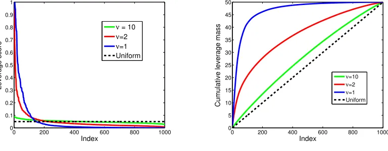
To compare the methods and see how they perform on inputs with different leverage scores, we generate test matrices using a method outlined in Ma et al. (2014, 2015). Set n= 1024 (to ensure, for simplicity, an integer power of 2 for the Hadamard transform) and p= 50, and let the number of samples drawn with replacement, r, be varied. X is then generated based on a t-distribution with different choices ofνto reflect different uniformity of leverage scores. Each row of X is selected independently with distribution Xi ∼ tν(Σ), where Σ
corresponds to an auto-regressive model with ν the degrees of freedom. The 3 values of
ν presented here are ν = 1 (highly non-uniform), ν = 2 (moderately non-uniform), and
ν = 10 (very uniform). See Figure 1 for a plot to see howνinfluences the uniformity of the leverage scores. For each setting, the simulation is repeated 100 times in order to average
0 200 400 600 800 1000
0 0.1 0.2 0.3 0.4 0.5 0.6 0.7 0.8 0.9 1
Index
Leverage score
ν = 10
ν=2
ν=1 Uniform
0 200 400 600 800 1000 0
5 10 15 20 25 30 35 40 45 50
Index
Cumulative leverage mass
ν=10
ν=2
ν=1
Uniform
Figure 1: Ordered leverage scores for different values ofν(a) and cumulative sum of ordered leverage scores for different values ofν (b).
over both the randomness in the sampling, and in the statistical setting, the randomness overy.
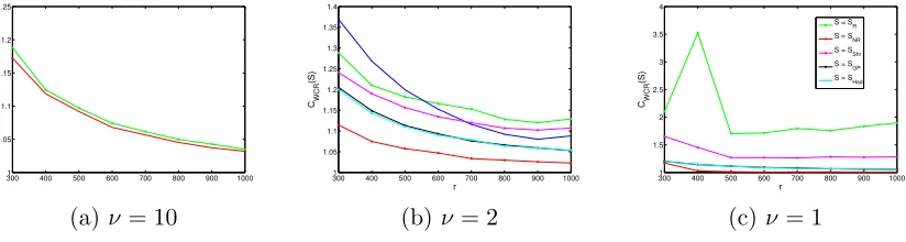
We first compare the sketching methods in the statistical setting by comparing CP E(S).
In Figure 2, we plot the average CP E(S) for the 6 subsampling approaches outlined above,
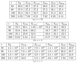
averaged over 100 samples for larger values of r between 300 and 1000. In addition, in Figure 3, we include a table for results on smaller values ofr between 80 and 200, to get a sense of the performance when r is close to p. Observe that in the large r setting,SN R is
clearly the best approach, out-performingSR, especially forν = 1. For smallr,
projection-based methods work better, especially forν = 1, since they tend to uniformize the leverage scores. In addition, SShr is superior compared to SN R, when r is small, especially when
ν = 1. We do not plot CRE(S) as it is simply a re-scaledCP E(S) to Lemma 1.
300 400 500 600 700 800 900 1000
1.5 2 2.5 3 3.5 4 4.5 5 5.5 r CRPE (S) S=SR
S = SNR
S =S Unif
S = SShr
S = S GP
S = SHad
300 400 500 600 700 800 900 1000
1 2 3 4 5 6 7 8 9 r CRPE (S)
S = S
R
S = SNR
S = S
Unif
S = SShr
S = S
GP
S = SHad
3000 400 500 600 700 800 900 1000 2 4 6 8 10 12 14 16 18 20 r CRPE (S)
S = S R S = SNR S = S
Shr S = SGP S = SHad
(a) ν= 10 (b) ν= 2 (c)ν = 1
Figure 2: Relative prediction efficiencyCP E(S) for large r.
r SR SN R SU nif SShr SGP SHad
80 39.8 38.7 37.3 39.8 35.5 40.0 90 27.8 27.2 27.2 27.2 26.1 27.4 100 22.4 22.1 22.7 22.2 21.3 23.1 200 8.33 7.88 8.51 7.62 8.20 8.14
(a) ν= 10
r SR SN R SU nif SShr SGP SHad
80 70.7 60.1 1.05×10² 73.3 36.5 39.8 90 45.6 34.6 66.2 44.7 26.7 28.2 100 35.1 25.9 52.8 33.8 22.1 22.5 200 9.82 5.54 15.3 9.17 7.59 7.81
(b)ν= 2
r SR SN R SU nif SShr SGP SHad
80 4.4×10⁴ 3.1×10⁴ 7.0×10³ 1.4×10⁴ 34.2 40.0 90 1.5×10⁴ 7.0×10³ 5.2×10³ 1.0×10⁴ 26.0 28.7 100 1.8×10⁴ 3.6×10³ 3.9×10³ 3.4×10³ 22.7 24.8 200 2.0×10² 34.0 5.2×10² 3.6×10² 7.94 7.84
(c) ν= 1
Figure 3: Relative prediction efficiencyCP E(S) for small r.
Overall, SN R, SR, and SShr compare very favorably to SU nif, which is consistent with
error. Furthermore, SR (which recall involves re-scaling) only increases the mean-squared
error, which is again consistent with the theoretical results. The effects are more apparent as the leverage score distiribution is more non-uniform (i.e., for ν= 1).
The theoretical upper bound in Theorems 1- 4 suggests thatCP E(S) is of the order nr,
independent of the leverage scores ofX, forS =SR as well asS =SHad and SGP. On the
other hand, the simulations suggest that for highly non-uniform leverage scores, CP E(SR)
is higher than when the leverage scores are uniform, whereas for S = SHad and SGP, the
non-uniformity of the leverage scores does not significantly affect the bounds. The reason that SHad and SGP are not significantly affected by the leverage-score distribution is that
the Hadamard and Gaussian projection has the effect of making the leverage scores of any matrix uniform Drineas et al. (2011). The reason for the apparent disparity whenS =SRis
that the theoretical bounds use Markov’s inequality which is a crude concentration bound. We suspect that a more refined analysis involving the bounded difference inequality would reflect that non-uniform leverage scores result in a larger CP E(SR).
3001 400 500 600 700 800 900 1000 1.05
1.1 1.15 1.2 1.25
300 400 500 600 700 800 900 1000
1 1.05 1.1 1.15 1.2 1.25 1.3 1.35 1.4
r
CWCR
(S)
3001 400 500 600 700 800 900 1000
1.5 2 2.5 3 3.5 4
r
CWCR
(S)
S = S R S = SNR
S = S Shr S = SGP
S = S Had
(a) ν= 10 (b) ν= 2 (c)ν = 1
Figure 4: Worst-case relative error CW C(S) for larger.
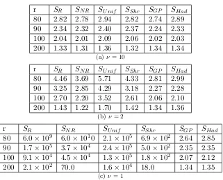
Finally, Figures 4 and 5 provide a comparison of the worst-case relative errorCW CE(S)
for large and small (r >200 andr ≤200, respectively) values ofr. Observe that, in general,
CW C(S) are much closer to 1 than CP E(S) for all choices of S. This reflects the scaling of p
n difference between the bounds. Interestingly, Figures 4 and 5 indicates that SN R still
tends to out-perform SR in general, however the difference is not as significant as in the
statistical setting.
5. Discussion and Conclusion
In this paper, we developed a framework for analyzing algorithmic and statistical criteria for general sketching matricesS∈Rr×napplied to the least-squares objective. As our analysis
makes clear, our framework reveals that the algorithmic and statistical criteria depend on different properties of the oblique projection matrix ΠUS = U(SU)†U, where U is the left singular matrix forX. In particular, the algorithmic criteria (WC) depends on the quantity supUT=0
kΠU
Sk2
kk2 , since in that case the data may be arbitrary and worst-case, whereas the
two statistical criteria (RE and PE) depends onkΠUSkF, since in that case the data follow
r SR SN R SU nif SShr SGP SHad
80 2.82 2.78 2.94 2.82 2.74 2.89 90 2.34 2.32 2.40 2.37 2.24 2.33 100 2.04 2.01 2.09 2.06 2.02 2.03 200 1.33 1.31 1.36 1.32 1.34 1.34
(a)ν= 10
r SR SN R SU nif SShr SGP SHad
80 4.46 3.69 5.71 4.33 2.81 2.99 90 3.25 2.85 4.29 3.18 2.27 2.28 100 2.70 2.20 3.52 2.61 2.06 2.10 200 1.43 1.22 1.70 1.42 1.34 1.36
(b)ν= 2
r SR SN R SU nif SShr SGP SHad
80 6.0×10⁹ 6.0×10¹⁰ 2.1×10⁵ 6.9×10² 2.64 2.85 90 1.7×10⁵ 3.7×10⁴ 2.4×10⁵ 5.0×10² 2.35 2.35 100 9.1×10⁴ 4.5×10⁴ 1.3×10⁵ 1.8×10² 2.07 2.12 200 2.1×10² 70.0 1.6×10⁴ 18.0 1.34 1.35
(c) ν= 1
Figure 5: Worst-case relative error CW C(S) for larger.
Using our framework, we develop upper bounds for 3 performance criteria applied to 4 sketching schemes. Our upper bounds reveal that in the regime where p < r n, our sketching schemes achieve optimal performance up to constants, in terms of WC and RE. On the other hand, the PE scales as nr meaningr needs to be close to (or greater than)nfor good performance. Subsequent lower bounds in Pilanci and Wainwright (2014) show that this upper bound can not be improved, but subsequent work by Pilanci and Wainwright (2014) as well as Lu and Foster (2014); Lu et al. (2013) provide alternate more sophisticated sketching approaches to deal with these challenges. Our simulation results reveal that for whenr is very close top, projection-based approaches tend to out-perform sampling-based approaches since projection-based approaches tend to be more stable in that regime.
Acknowledgement. We would like to thank the Statistical and Applied Mathematical Sciences Institute and the members of its various working groups for helpful discussions.
Appendix A. Auxiliary Results
In this section, we provide proofs of Lemma 1 and an intermediate result we will later use to prove the main theorems.
A.1 Proof of Lemma 1
Recall thatX =UΣVT, whereU ∈Rn×p, Σ∈
Rp×p and V ∈Rp×p denote the left singular
matrix, diagonal singular value matrix and right singular matrix respectively. First we show thatkY −XβOLSk22=kk22. To do so, observe that
kY −XβOLSk22 = kY −UΣVTβOLSk22,
and setδOLS = ΣVTβOLS. It follows that δOLS =UTY. Hence
kY −XβOLSk22=kY −ΠUYk22,
where ΠU =U UT. For every Y ∈Rn, there exists a unique δ ∈ Rp and ∈Rn such that
UT= 0 and Y =U δ+. Hence
kY −XβOLSk22=k(In×n−ΠU)k22 =kk22,
where the final equality holds since ΠU= 0.
Now we analyzekY −XβSk22. Observe that
kY −XβSk22 =kY −ΠSUYk22,
where ΠUS =U(SU)†S. Since Y =U δ+, it follows that
kY −XβSk22 = kU(Ip×p−(SU)†SU)δ+ (In×n−ΠSU)k22
= k(Ip×p−(SU)†SU)δk22+k(In×n−ΠSU)k22
= k(Ip×p−(SU)†SU)δk22+kk22+kΠSUk22.
Therefore for allY:
CW C(S) =
kY −XβSk22
kY −XβOLSk22
= 1 +k(Ip×p−(SU)
†SU)δk2
2+kΠUSk22
kk2
2
,
where UT= 0. Taking a supremum over Y and consequently over and δ completes the proof for CW C(S).
Now we turn to the proof for CP E(S). First note that
E[kX(βOLS−β)k22] =E[kU UTY −UΣVTβk22].
Under the linear model Y =UΣVTβ+,
Since E[T] =In×n, it follows that
E[kX(βOLS −β)k22] =E[kΠUk22] =kΠUk2F =p.
ForβS, we have that
E[kX(βS−β)k22] =E[kΠUSY −UΣVTβk22] = E[k(U(I−(SU)†SU)ΣVTβ+ ΠUSk22]
= k(Ip×p−(SU)†SU)ΣVTβk22+E[kΠUSk22]
= k(Ip×p−(SU)†SU)ΣVTβk22+kΠUSk2F.
Hence CP E(S) = 1/p(k(Ip×p−(SU)†SU)ΣVTβk22+kΠUSk2F) as stated.
For CRE(S), the mean-sqaured error for δOLS andδS are
E[kY −XβOLSk22] = E[k(I−ΠU)k22]
= kI−ΠUk2
F =n−p,
and
E[kY −XβSk22] = k(Ip×p−(SU)†SU)ΣVTβk22+E[k(I−ΠUS)k22]
= k(Ip×p−(SU)†SU)ΣVTβk22+ trace((I −ΠS)T(I−ΠS))
= k(Ip×p−(SU)†SU)ΣVTβk22+ trace(I)−2trace(ΠS) +kΠSk2F
= k(Ip×p−(SU)†SU)ΣVTβk22+n−2p+kΠSk2F
= k(Ip×p−(SU)†SU)ΣVTβk22+n−p+kΠSk2F −p.
Hence,
CRE(S) =
n−p+k(Ip×p−(SU)†SU)ΣVTβk22+kΠSk2F −p
n−p
= 1 +k(Ip×p−(SU)
†SU)ΣVTβk2
2+kΠSk2F −p
n−p
= 1 +CP E(S)−1
n/p−1 .
A.2 Intermediate Result
In order to provide a convenient way to parameterize our upper bounds for CW C(S),
CP E(S), and CRE(S), we introduce the following three structural conditions on S. Let
˜
σmin(A) denote the minimum non-zero singular value of a matrixA.
• The first condition is that there exists an α(S)>0 such that
˜
σmin(SU)≥α(S). (12)
• The second condition is that there exists a β(S) such that
sup
, UT=0
kUTSTSk
2
kk2
• The third condition is that there exists aγ(S) such that
kUTSTSkF ≤γ(S). (14)
Note that the structural conditions defined byα(S) andβ(S) have been defined previously as Eqn. (8) and Eqn. (9) in Drineas et al. (2011).
Given these quantities, we can state the following lemma, the proof of which may be found in Section A.2. This lemma provides upper bounds forCW C(S),CP E(S), andCRE(S)
in terms of the parametersα(S),β(S), andγ(S).
Lemma 2 For α(S) and β(S), as defined in Eqn.(12) and (13),
CW C(S)≤1 + sup
δ∈Rp,UT=0
k(Ip×p−(SU)†(SU))δk22
kk2
2
+β
2(S)
α4(S).
For α(S) andγ(S), as defined in Eqn. (12) and (14),
CP E(S)≤
k(Ip×p−(SU)†SU)ΣVTβk22
p +
γ2(S)
α4(S).
Furthermore,
CRE(S)≤1 +
p n
k
(Ip×p−(SU)†SU)ΣVTβk22
p +
γ2(S)
α4(S)
.
Again, the terms involving (SU)†SU are a “bias” that equal zero for rank-preserving sketch-ing matrices. In addition, we emphasize that the results of Lemma 1 and Lemma 2 hold for arbitrary sketching matrices S. In Appendix A.3, we bound α(S), β(S) and γ(S) for several different randomized sketching matrices, and this will permit us to obtain bounds on CW C(S), CP E(S), andCRE(S). For the sketching matrices we analyze, we prove that
the bias term is 0 with high probability.
A.3 Proof of Lemma 2
Note that ΠUS =U(SU)†S. Let rank(SU) = k < p, and the singular value decomposition isSU = ˜UΣ ˜˜VT, where ˜Σ∈Rk×k is a diagonal matrix with non-zero singular values of SU.
Then,
kΠUSk2
2
kk2
2
= kU(SU)
†Sk2
2
kk2
2
= k(SU)
†Sk2
2
kk2
2
= k ˜
VΣ˜−1U˜TSk2
2
kk2
2
= kV˜Σ˜
−2V˜TV˜Σ ˜˜UTSk2
2
kk2
2
where we have ignored the bias term which remains unchanged. Note that ˜VΣ˜−2V˜T α−2(S)Ip×p and ˜VΣ ˜˜UT = (SU)T =UTST. Hence,
kΠUSk2
2
kk2
2
= kV˜Σ˜
−2V˜TV˜Σ ˜˜UTSk2
2
kk2
2
≤ kU
TSTSk2 2
α4(S)kk2
2
= β
2(S)
α4(S)kk2
2
,
and the upper bound onCW C(S) follows.
Similarly,
kΠUSk2F =kU(SU)†SkF2 =k(SU)†Sk2F =kV˜Σ˜−2V˜TV˜Σ ˜˜UTSk2F ≤α−4(S)kUTSTSk2F
and the upper bound onCP E(S) follows.
Appendix B. Proof of Main Theorems
The proof techniques for all of four theorems are similar, in that we use the intermediate result Lemma 2 and bound the expectations ofα(S),β(S), andγ(S) for eachS, then apply Markov’s inequality to develop high probability bounds.
B.1 Proof of Theorem 1
First we bound α2(SR) by using existing results in Drineas et al. (2011). In particular
applying Theorem 4 in Drineas et al. (2011) with β = 1−θ, A=UT,= √1
2 and δ= 0.1
provides the desired lower bound on α(SR) and ensures that the ”bias” term in Lemma 2
is 0 since rank(SRU) =p.
To upper bound β(SR), we first upper bound its expectation, then apply Markov’s
inequality. Using the result of Table 1 (second row) of Drineas et al. (2006a) withβ= 1−θ:
E[kUTSRTSRk22]≤
1 (1−θ)rkU
Tk2
Fkk22=
p
(1−θ)rkk
2 2.
Applying Markov’s inequality,
kUTSRTSRk22≤
11p
(1−θ)rkk
2 2,
Finally we bound γ(SR):
1
p[kU
TST
RSRk2F] =
1
p[trace(U
T(ST
RSR)2U)]
= 1 p p X j=1 n X i=1 n X k=1
UijUkj[(SRTSR)2]ki
= 1 p p X j=1 n X i=1
Uij2[SRTSR]2ii
= 1
p
n
X
i=1
`i[SRTSR]2ii,
where the second last equality follows since [SRTSR]2ki = 0 for k 6= i and the final equality
follows since `i = Ppj=1Uij2. First we upper bound E[γ(SR)] and then apply Markov’s
inequality. Recall that [SR]ki = √rpi1 σki where P(σki = +1) =pi. Then,
1
p
n
X
i=1
`iE([SRTSR]2ii]) =
1
r2p
n
X
i=1
`i
p2i
r X m=1 r X `=1
E[σ2miσ2`i]
= 1
r2p
n
X
i=1
`i
p2i
r X m=1 r X `=1
E[σmiσ`i]
= 1
r2p
n
X
i=1
`i
p2i[(r
2−r)p2
i +rpi]
= 1
r2p
n
X
i=1
(`i(r2−r) +r
`i
pi
)]
= 1−1
r + 1 rp n X i=1 `i pi .
Substituting pi = (1−θ)`ip +θqi completes the upper bound on E[γ(SR)]:
1−1
r + 1 rp n X i=1 `i pi
= 1−1
r + 1 rp n X i=1 `i
(1−θ)`ip +θqi
≤ 1−1
r + 1 r n X i=1 1 1−θ
≤ 1−1
r +
n
(1−θ)r
≤ 1 + n
(1−θ)r.
Using Markov’s inequality,
P |γ(SR)−E[γ(SR)]| ≥10E[γ(SR)]
and consequently γ(SR) ≤ 11(1 + (1−nθ)r) with probability greater than 0.9. The final
probability of 0.7 arises since we simultaneously require all three bounds to hold which hold with probability 0.93 >0.7. Applying Lemma 2 in combination with our high probability bounds forα(SR), β(SR) andγ(SR) completes the proof for Theorem 1.
B.2 Proof of Theorem 2
Define S =
q
k
rSN R where SN R is the sampling matrix without re-scaling. Recall the
k-heavy hitter leverage-score assumption. Since Pn
i=k+1`i ≤
p
10r,
Pn
i=k+1pi ≤ 1
10r (recall
pi = `ip). Hence the probability that a sample only contains theksamples with high leverage
score is:
(1− 1
10r)
r ≥1− 1
10 = 0.9.
For the remainder of the proof, we condition on the eventA that only the rows with thek
largest leverage scores are selected. Let ˜U ∈Rk×p be the sub-matrix ofU corresponding to
the topk leverage scores.
Let W = E[STS] ∈ Rk×k. Since kc ≤pi ≤ Ck for all 1 ≤ i≤ k, cIk×k W CIk×k.
Furthermore sincePn
i=k+1`i ≤
p
10r, 0.9Ip×pU˜TU˜ Ip×p.
First we lower boundα2(SN R). Applying Theorem 4 in Drineas et al. (2011) withβ=C,
A= ˜UTW1/2,= 2c and δ = 0.1 ensures that as long asr ≥c0plog(p) for sufficiently large
c0,
kU˜TWU˜−U˜TSTSUk˜ op≤
c
2C,
with probability at least 0.9. Since ˜UTWU˜ 3c
4, ˜U
TSTSU˜ c
4. Therefore with probability
at least 0.9,
α2(SN R)≥
cr
4Ck.
Next we bound β(SN R). Since S =
q
k
rSN R, if we condition on A, only the leading k
leverage scores are selected and let ˜U ∈Rk×p be the sub-matrix ofU corresponding to the
top k leverage scores. Using the result of Table 1 (second row) of Drineas et al. (2006a) withβ = 1:
E[kUTSN RT SN Rk22] =
r2
k2E[kU
TSTSk2 2] =
r2
k2E[kU˜
TSTSk2 2]≤
r2
k2kU˜
Tk2 2kk22 ≤
pr2
k2 kk
2 2.
Applying Markov’s inequality,
kUTSN RT SN Rk22 ≤
11pr2
k2 kk
2 2,
Finally we bound γ(SN R):
trace( ˜UT(STS)2U˜)/p = 1
p
n
X
i=1
[STS]2ii
p
X
j=1
˜
Uij2
= 1
p
k
X
i=1
`i[S T
S]2ii
≤ Ck r k X i=1 1 r( r X m=1
σmi2 )2,
where the last step follows since `i ≤ Cpk for 1 ≤ i ≤ k and 0 otherwise. Now taking
expectations:
1
rE[
k X i=1 ( r X m=1
σmi)2] =
1 r k X i=1 r X `=1 r X m=1
E[σ`iσmi]
≤ C 2 r k X i=1 (r
2−r
k2 +
r
k)
= C2(r−1
k + 1)
≤ C2(r
k+ 1).
SinceSN R =
q
k
rS,E[trace(UT(SN RT SN R)2U)/p]≤C2(1 + k
r). Applying Markov’s
inequal-ity,
trace(UT(SN RT SN R)2U)/p≤11C2(1 +
k
r),
with probability at least 0.9. The probability of 0.6 arises since 0.94 >0.6. Again, using Lemma 2 completes the proof for Theorem 2.
B.3 Proof of Theorem 3
First we bound the smallest singular value of SSGP(U). Using standard results for bounds
on the eigenvalues of sub-Gaussian matrices (see Proposition 2.4 in Rudelson and Vershynin (2009)), each entry ofA∈Rr×n is an i.i.d. zero-mean sub-Gaussian matrix:
P( inf
kxk2=1
1 √ rkAxk 2 2≤ 1 √
2)≤nexp(−cr).
Hence, providedcr ≥2 logn,
α(SSGP)≥
1
√
2,
Next we boundβ(SSGP). SinceUT= 0,kUTSSGPT SSGPk22=kUT(SSGPT SSGP−In×n)k22.
Therefore
kUTSSGPT SSGPk22 =
p X j=1 n X i=1 n X k=1
Uij(SSGPT SSGP −In×n)ikk
2 = p X j=1 n X i=1 n X k=1 n X m=1 n X `=1
UijUmj(SSGPT SSGP −In×n)ik(SSGPT SSGP −In×n)m`k`.
First we boundE[kUTSSGPT SSGPk22].
E[kUTSTSGPSSGPk22] =
p X j=1 n X i=1 n X k=1 n X m=1 n X `=1
UijUmjE[(SSGPT SSGP−In×n)ik(SSGPT SSGP−In×n)m`]k`.
Recall that SSGP ∈ Rr×n, [SSGP]si = Xsi√r where Xsi are i.i.d. sub-Gaussian random
vari-ables with mean 0 and sub-Gaussian parameter 1. Hence
E[(SSGPT SSGP −In×n)ik(SSGPT SSGP −In×n)m`] =
1
r(I(i=k)I(`=m) +E[XiXjX`Xm]),
whereXi, Xk, X` andXm are i.i.d . sub-Gaussian random variables. Therefore
E[kUTSTSGPSSGPk22] =
1 r p X j=1 n X i=1 n X k=1 n X m=1 n X `=1
UijUmj(I(i=k)I(`=m)+E[XiXkX`Xm])k`.
First note that I(i = k)I(` = m) +E[XiXkX`Xm] = 0 unless i = k and ` = m, or i= `
and k =` or any other combination of two pairs of variables have the same index. When
i=k=`=m,I(i=k)I(`=m) +E[XiXkX`Xm] = 1 +E[Xi4]≤2, since for sub-Gaussian
random variables with parameter 1, E[Xi4]≤1 and 1 r p X j=1 n X i=1 n X k=1 n X m=1 n X `=1
UijUmj(I(i=k)I(`=m) +E[XiXkX`Xm])k` =
1 r p X j=1 n X i=1
Uij22i(1 +E[Xi4])
≤ 2 r p X j=1 n X i=1
Uij22i
≤ 2
r
p
X
j=1
Uij2kk22
= 2p
r kk
2 2.
When i=k and`=m butk6=`,I(i=k)I(`=m) +E[XiXkX`Xm] = 2 and
p X j=1 n X i=1 n X k=1 n X m=1 n X `=1
UijUmj(I(i=k)I(`=m)+E[XiXkX`Xm])k`= 2
p X j=1 n X i=1 n X `=1
since UT = 0. Using similar logic when the two pairs of variables are not identical, the sum is 0, and hence
E[kUTSSGPT SSGPk22]≤
2p
r kk
2 2,
for all such thatUT= 0. Applying Markov’s inequality,
kUTSSGPT SSGPk22 ≤
22p
r kk
2 2,
with probability greater than 0.9. Thereforeβ(SSGP)≤
q
22p
r with probability at least 0.9.
Now we bound γ(SSGP) =kUTSSGPT SSGPkF2 = trace(UT(STSGPSSGP)2U)/p:
trace(UT(SSGPT SSGP)2U)/p =
1 p p X j=1 n X i=1 n X k=1
[(STSGPSSGP)2]ikUijUkj
= 1 pr2 p X j=1 n X i=1 n X k=1 n X v=1 r X m=1 r X `=1
UijUkjXmvXmiX`vX`k.
First we bound the expectation:
E[trace(UT(SSGPT SSGP)2U)/p] =
1 pr2 p X j=1 n X i=1 n X k=1 n X v=1 r X m=1 r X `=1
E[XmvXmiX`vX`k]
= 1 pr2 p X j=1 n X i=1 n X k=1 n X v=1
(r2−r)UijUkjE[XvXi]E[XvXk] +rE[Xv2XiXk]
= 1 pr2 p X j=1 n X i=1
(r2−r)Uij2(E[Xi2])2+
1 pr2 p X j=1 n X i=1 n X v=1
rUij2E[Xv2Xi2]
= 1 pr2 p X j=1 n X i=1
(r2−r)Uij2σ4+ 1
pr2 p X j=1 n X i=1 n X v=1
rUij2E[Xv2Xi2]
= 1−1
r +
µ4
σ4r +
n−1
r
≤ 1 +3
r +
n−2
r
= 1 +(n+ 1)
r .
Applying Markov’s inequality,
γ(SSGP)≤11(1 +
(n+ 1)
r ),
B.4 Proof of Theorem 4
ForS =SHad we use existing results in Drineas et al. (2011) to lower boundα2(SHad) and
β(SHad) and then upper boundγ(SHad). Using Lemma 4 in Drineas et al. (2011) provides
the desired lower bound on α2(S
Had).
To upper bound β(SHad), we use Lemma 5 in Drineas et al. (2011) which states that:
kUTST
HadSHadk22≤
20dlog(40nd)kk2 2
r ,
with probability at least 0.9.
Finally to bound γ(SHad) recall that SHad = SU nifHD, where SU nif is the uniform
sampling matrix, Dis a diagonal matrix with±1 entries and H is the Hadamard matrix:
1
p[kU
TST
HadSHadk2F] =
1
p[trace(U
T(ST
HadSHad)2U)]
= 1
p[trace(U
T(DTHTST
U nifSU nifHD)2U)]
= 1
p[trace(U
TDTHTST
U nifSU nifHDDTHTSU nifT SU nifHDU)]
= 1
p[trace(U
TDTHT(ST
U nifSU nif)2HDU)]
= 1
p
p
X
j=1
n
X
i=1
n
X
k=1
[HDU]ij[HDU]kj[(SU nifT SU nif)2]ki
= 1
p
p
X
j=1
n
X
i=1
[HDU]2ij[SU nifT SU nif]2ii.
Using Lemma 3 in Drineas et al. (2011), with probability greater than 0.95,
1
p
p
X
j=1
[HDU]2ij ≤ 2 log(40np)
n .
In addition, we have that
1
p[kU
TST
HadSHadk2F] =
1
p
p
X
j=1
n
X
i=1
[HDU]2ij[SU nifT SU nif]2ii
≤ 2 log(40np) n
n
X
i=1
[SU nifT SU nif]2ii.
n
X
i=1
E([SU nifT SU nif]2ii]) =
n2
r2
n
X
i=1
r
X
m=1
r
X
`=1
E[σmi2 σ2`i]
= n
2
r2
n
X
i=1
r
X
m=1
r
X
`=1
E[σmiσ`i]
= n
2
r2
n
X
i=1
[r
2−r
n2 +
r
n]
= n
2
r2[
r2−r
n +r]
= n−n
r +
n2
r
≤ n+n
2
r .
Using Markov’s inequality, with probability greater than 0.9,
n
X
i=1
[STU nifSU nif]2ii≤10(n+
n2
r ),
which completes the proof.
References
H. Avron, P. Maymounkov, and S. Toledo. Blendenpik: Supercharging LAPACK’s least-squares solver. SIAM Journal on Scientific Computing, 32:1217–1236, 2010.
C. Boutsidis and A. Gittens. Improved matrix algorithms via the subsampled randomized Hadamard transform. SIAM Journal of Matrix Analysis and Applications, 34:1301–1340, 2013.
S. Chatterjee and A. S. Hadi. Influential observations, high leverage point, and outliers in linear regression. Statistical Science, 1(3):379–416, 2006.
S. Chatterjee and A.S. Hadi. Sensitivity Analysis in Linear Regression. John Wiley & Sons, New York, 1988.
K. L. Clarkson and D. P. Woodruff. Low rank approximation and regression in input sparsity time. InProceedings of the 45th Annual ACM Symposium on Theory of Computing, pages 81–90, 2013.
P. Drineas, R. Kannan, and M. W. Mahoney. Fast Monte Carlo algorithms for matrices I: approximating matrix multiplication. SIAM J. Comput., 36:132–157, 2006a.
P. Drineas, M.W. Mahoney, and S. Muthukrishnan. Sampling algorithms for `2 regression
and applications. InProceedings of the 17th Annual ACM-SIAM Symposium on Discrete
P. Drineas, M. W. Mahoney, S. Muthukrishnan, and T. Sarlos. Faster least squares approx-imation. Numerical Mathematics, 117:219–249, 2011.
P. Drineas, M. Magdon-Ismail, M. W. Mahoney, and D. P. Woodruff. Fast approximation of matrix coherence and statistical leverage. Journal of Machine Learning Research, 13: 3475–3506, 2012.
G. H. Golub and C. F. Van Loan. Matrix Computations. Johns Hopkins University Press, Baltimore, 1996.
F. R. Hampel, E. M. Ronchetti, P. J. Roisseeuw, and W. A. Stahel. Robust Statisitcs: The
Approach Based on Influence Functions. John Wiley & Sons, New York, 1986.
A. Hedayat and W. D. Wallis. Hadamard matrices and their applications. Annals of
Statistics, 6(6):1184–1238, 1978.
D.C. Hoaglin and R.E. Welsch. The hat matrix in regression and ANOVA. The American
Statistician, 32(1):17–22, 1978.
P. J. Huber and E. M. Ronchetti. Robust Statisitcs. John Wiley & Sons, New York, 1981.
W. B. Johnson and J. Lindenstrauss. Extensions of Lipschitz mappings into a Hilbert space. volume 26, pages 189–206, 1984.
E. L. Lehmann. Elements of Large-Sample Theory. Springer Verlag, New York, 1998.
Y. Lu and D. P. Foster. Fast ridge regression with randomized principal component analysis and gradient descent. In Proceedings of NIPS 2014, 2014.
Y. Lu, P. S. Dhillon, D. P. Foster, and L. Ungar. Faster ridge regression via the subsampled randomized Hadamard transform. In Proceedings of NIPS 2013, 2013.
P. Ma, M. W. Mahoney, and B. Yu. A statistical perspective on algorithmic leveraging. In
Proceedings of the 31st International Conference on Machine Learning, 2014.
P. Ma, M. W. Mahoney, and B. Yu. A statistical perspective on algorithmic leveraging.
Journal of Machine Learning Research, 16:861–911, 2015.
M. W. Mahoney. Randomized algorithms for matrices and data. Foundations and Trends in Machine Learning. NOW Publishers, Boston, 2011. Also available at: arXiv:1104.5557.
M. W. Mahoney and P. Drineas. CUR matrix decompositions for improved data analysis.
Proc. Natl. Acad. Sci. USA, 106(3):697–702, 2009.
X. Meng and M. W. Mahoney. Low-distortion subspace embeddings in input-sparsity time and applications to robust linear regression. In Proceedings of the 45th Annual ACM
Symposium on Theory of Computing, pages 91–100, 2013.