Expectation Consistent Approximate Inference
Manfred Opper [email protected]
ISIS, School of Electronics and Computer Science University of Southampton
SO17 1BJ, United Kingdom
Ole Winther [email protected]
Informatics and Mathematical Modelling Technical University of Denmark DK-2800 Lyngby, Denmark
Editor:Michael I. Jordan
Abstract
We propose a novel framework for approximations to intractable probabilistic models which is based on a free energy formulation. The approximation can be understood as replacing an average over the original intractable distribution with a tractable one. It requires two tractable probability distributions which are made consistent on a set of moments and encode different features of the original intractable distribution. In this way we are able to use Gaussian approximations for models with discrete or bounded variables which allow us to include non-trivial correlations. These are neglected in many other methods. We test the framework on toy benchmark problems for binary variables on fully connected graphs and 2D grids and compare with other methods, such as loopy belief propagation. Good performance is already achieved by using single nodes as tractable substructures. Significant improvements are obtained when a spanning tree is used instead.
1. Introduction
Recent developments in data acquisition and computational power have spurred an increased interest in flexible statistical Bayesian models in many areas of science and engineering. Inference in probabilistic models is in many cases intractable; the computational cost of marginalization operations can scale exponentially in the number of variables or require integrals over multivariate non-tractable distributions. In order to treat systems with a large number of variables, it is therefore necessary to use approximate polynomial complexity inference methods.
a bound. The most important tractable families of distributions in the variational bound approximation are multivariate Gaussians and distributions often in the exponential family which factorize in the marginals of all or for certain disjoint groups of variables (Attias, 2000) (this is often called a mean–field approximation). The use of multivariate Gaussians makes it possible to retain a significant amount of correlation between variables in the approximation. However, their application in the variational bound approximation is limited to distributions of continuous variables which have the entire real space as their natural domain. This is due to the fact that the KL divergence would diverge for distributions with non-matching support. Hence, in a majority of those applications, where random variables with constrained values (such as Boolean ones) appear, variational distributions of the mean field type have to be chosen. However, such factorizing approximations have the drawback that correlations are neglected and one often observes that fluctuations are underestimated (MacKay, 2003; Opper and Winther, 2004).
Recently, a lot of effort has been devoted to the development of approximation tech-niques which give an improved performance compared to the variational bound approxi-mation. Thomas Minka’s Expectation Propagation(EP) approach (Minka, 2001a,b) seems to provide a general framework from which many of these developments can be re-derived and understood. EP is based on a dynamical picture where factors—their product form-ing a global tractable approximate distribution—are iteratively optimized. In contrast to the variational bound approach, the optimization proceedslocallyby minimizing KL diver-gences between appropriately definedmarginal distributions. Since the resulting algorithm can be formulated in terms of the matching of marginal moments, this would not rule out factorizations where discrete distributions are approximated by multivariate Gaussians. However, such a choice seems to be highly unnatural from the derivation of the EP ap-proximation (by the infinite KL measure) and has to our knowledge not been suggested so far (Minka, private communication). Hence, in practice, the correlations between discrete variables have been mainly treated using tree-based approximations. This includes the cel-ebrated Bethe-Kikuchi approach (Yedidia et al., 2001; Yuille, 2002; Heskes et al., 2003), for EP interpretations see Minka (2001a,b) and Minka and Qi (2004). For a variety of re-lated approximations within statistical physics see Suzuki (1995). However, while tree-type approximations often work well for sparsely connected graphs they become inadequate for inference problems in a dense graph regardless of the type of variables.
Although one algorithmic realization of our method can be given an EP-style interpretation (Csat´o et al., 2002), we believe that it is more natural and more powerful to base the derivation on a framework of optimizing a free energy approximation. This not only has the advantage of providing a simple and clear way for adapting the model parameters within the empirical Bayes framework, but also motivates different practical optimization algorithms among which the EP–style may not always be the best choice.
Our paper is organized as follows: Section 2 motivates approximate inference and ex-plains the notation. The expectation consistent (EC) approximation to the free energy is derived in Section 3. Examples for EC free energies are given in Section 4. The algorithmic issues are treated in Section 5, simulations in Section 6 and finally we conclude in Section 7.
2. Motivation: Approximate Inference
We consider the problem of computing expectations, i.e. certain sums or integrals involv-ing a probability distribution with density p(x) for a vector of random variables x = (x1, x2, . . . , xN). We assume that such computations are considered intractable, either
be-cause the necessary sums are over a too large number of variables or bebe-cause multivariate integrals cannot be evaluated exactly. A further complication might occur when the density itself is expressed by a non-normalized multivariate functionf(x), say, equal to the product of a prior and a likelihood, which requires further normalization, i.e.
p(x) = 1
Zf(x) , (1)
where the partition function Z must be obtained by the (intractable) summation or inte-gration of f: Z = R
dxf(x). In a typical scenario, f(x) is expressed as a product of two functions
f(x) =fq(x)fr(x) (2)
withfq,r(x)≥0, wherefqis “simple” enough to allow for tractable computations. The goal
is to approximate the “complicated” part fr(x) by replacing it with a “simpler” function,
say of some exponential form
exp λTg(x)
≡exp
K
X
j=1
λjgj(x)
. (3)
We have used the same vector notation forg-vectors as for the random variablesx, however one should note that vectors will often have different dimensionalities, i.e. K 6= N. The vector of functions g is chosen in such a way that the desired sums or integrals can be calculated in an efficient way and the parametersλare adjusted to optimize certain criteria. Hence, the word tractability should always be understood as relative to some approximating set of functions g.
Our framework of approximation will be restricted to problems, where both parts fq
and fr can be considered as tractable relative to some suitable g, and the intractability
of the density p arises from forming their product.2 In such a case, one may alternatively retain fr but replace fq by an approximation of the form eq. (3). One would then end up
with two types of approximations
q(x) = 1 Zq(λq)
fq(x) exp λTqg(x)
(4)
r(x) = 1 Zr(λr)
fr(x) exp λTrg(x)
(5)
for the same density, where Zq(λq) =
R
dx fq(x) exp λTqg(x)
. We will not assume that either choiceq andris a reasonably good approximation for the global joint densityp(x) as we do in the variational bound approximation. In fact, later we will apply our method to the case of Ising variables, where the KL divergence between one of them andpis even infinite! Though, suitable different marginalizations of q and r can give quite accurate answers for important marginal statistics.
Take, as an example, the density p(x) =f(x)/Z =fq(x)fr(x)/Z—with respect to the
Lebesgue measure in RN—with
fq(x) =
Y
i
ψi(xi) (6)
fr(x) = exp
X
i<j
xiJijxj+
X
i
θixi
, (7)
where, in order to have a nontrivial problem,ψi should be a non-Gaussian function. We will
name this the quadratic model. Usually there will be an ambiguity in the choice of factor-ization, e.g. we could have included exp (P
iθixi) as a part offq(x). One may approximate
p(x) by a factorizing distribution, thereby replacingfr(x) by some function which factorizes
in the components xi. Alternatively, one can consider replacing fq(x) by a Gaussian
func-tion to make the whole distribufunc-tion Gaussian. Both approximafunc-tions are not ideal. The first completely neglects correlations of the variables but leads to marginal distributions of the xi, which might qualitatively resemble the non-Gaussian shape of the true marginal. The
second one neglects the non-Gaussian effects but incorporates correlations which might be used in order to approximate the two variable covariance functions. While within the varia-tional bound approximation, both approximations appear independent from each other we will, in the following develop an approach for combining two complimentary approximations which “communicate” by matching the corresponding expectations of the functionsg(x).
2.1 Notation
densityp by brackets
hh(x)i= Z
dxp(x)h(x) = 1 Z
Z
dxf(x)h(x), (8)
where, in cases of ambiguity, the density will appear as a subscript, like in hh(x)ip. One of
the strengths of our formalism is to allow for a treatment of discrete and continuous random variables within the same approach.
Example: Ising variables Discrete random variables can be described using Dirac dis-tributions in the densities. For examples, the density of N independent Ising variables xi ∈ {−1,+1}which occur with equal probabilities (one-half) has the density
p(x) =
N
Y
i=1
1
2δ(xi+ 1) + 1
2δ(xi−1)
. (9)
3. Expectation Consistent Free Energy Approximation
In this section we will derive an approximation for−lnZ, the negative log-partition function also called the (Helmholtz) free energy. We will use an approximating distribution q(x) of the type eq. (4) and split the exact free energy into a corresponding part−lnZqplus a rest
which will be further approximated. The split is obtained by writing
Z = Zq
Z Zq =Zq
R
dxfr(x)fq(x) exp (λq−λq)Tg(x)
R
dxfq(x) expλTqg(x)
(10)
= Zq
fr(x) exp −λTqg(x)
q ,
where
Zq(λq) =
Z
dxfq(x) exp λTqg(x)
. (11)
This expression can be used to derive a variational bound to the free energy−lnZ. Applying Jensen’s inequality lnhf(x)i ≥ hlnf(x)i we arrive at
−lnZ ≤ −lnZvar =−lnZq− hlnfr(x)iq+λTq hg(x)iq . (12)
The optimal value forλq is found by minimizing this upper bound.
Our new approximation is obtained by arguing thatone may do better by retaining the
fr(x) exp −λTqg(x)
expressionin eq. (10) but instead changing the distribution we use in averaging. Hence, we replace the average with respect to q(x) with an average using a distributions(x) containing the same exponential form
s(x) = 1 Zs(λs)
exp λTsg(x) .
Given a sensible strategy for choosing the parameters λs and λq, we expect that this
the closer the result will to the exact partition function. It is difficult to make this state-ment quantitative and general. However, the method gives nontrivial results for a variety of cases where the variational bound would be simply infinite! This always happens, when fq is Gaussian andfr vanishes on a set which has nonzero probability with respect to the
density fq. Examples are when fr is discrete or contains likelihoods which vanish in
cer-tain regions as in noise-free Gaussian process classifiers (Opper and Winther, 1999). Our approximation is further supported by the fact that for specific choices of fr and fq it is
equivalent to the adaptive TAP (ADATAP) approximation (Opper and Winther, 2001a,b). ADATAP (unlike the variational bound) gives exact results for certain statistical ensembles of distributions in an asymptotic (thermodynamic) limit studied in statistical physics.
Usingsinstead ofq, we arrive at the approximation for−lnZ which depends upon two sets of parametersλq andλs:
−lnZEC(λq,λs) = −lnZq−ln
fr(x) exp −λTqg(x)
s
= −ln Z
dxfq(x) exp λTqg(x)
−ln Z
dxfr(x) exp (λs−λq)Tg(x)
+ ln Z
dxexp λTsg(x)
. (13)
Here we have utilized our additional assumption, that also fr is tractable with respect to
the exponential family and thus Zr=
R
dxfr(x) exp (λs−λq)Tg(x)
can be computed in polynomial time. Eq. (13) leaves two sets of parameters λq and λs to be determined. We
expect that eq. (13) is a sensible approximation as long ass(x) shares some key properties with q, for which we choose thematching of the moments hg(x)iq =hg(x)is. This will fix
λs as a function of λq. Second, we know that the exact expression eq. (10) is independent
of the value of λq. If the replacement of q(x) by s(x) yields a good approximation, one
would still expect that eq. (13) is a fairly flat function of λq (after eliminating λs) in a
certain region. Hence, it makes sense to require that an optimized approximation should make eq. (13)stationarywith respect to variations of λq. This does not imply that we are
expecting a local minimum of eq. (13), see also section 3.1, but saddle points could occur. Since we are not after a bound on the free energy, this is not necessarily a disadvantage of the method. Readers who feel uneasy with this argument, might find the alternative, dual derivation (using the Gibbs free energy) in appendix B more appealing.
Both conditions can be summarized by the expectation consistency(EC) conditions ∂lnZEC
∂λq
= 0 : hg(x)iq=hg(x)ir (14) ∂lnZEC
∂λs
= 0 : hg(x)ir=hg(x)is (15) for the three approximating distributions
q(x) = 1 Zq(λq)
fq(x) exp(λTqg(x)) (16)
r(x) = 1 Zr(λr)
fr(x) exp(λTrg(x)) with λr =λs−λq (17)
s(x) = 1 Zr(λs)
The corresponding EC approximation of the free energy is then
−lnZ ≈ −lnZEC=−lnZq(λq)−lnZr(λs−λq) + lnZs(λs) (19)
whereλq and λs are chosen such that the partial derivatives of the right hand side vanish.
3.1 Properties of the EC approximation
Invariances Although our derivation started with approximating one of the two factors fq andfrby an exponential, the final approximation is completely symmetric in the factors
fqandfr. We could have chosen to defineqin terms offr and still got the same final result.
Iff contains multiplicative terms which are of the form exp λTg(x)
for some fixedλ, we are free to include them either in fq or fr without changing the approximation. This can
be easily shown by redefiningλq →λq±λ.
Derivatives with respect to parameters. The following is a useful result about the derivative of −lnZEC with respect to a parameter t in the density p(x). Setting λ = (λq,λs), we get
dlnZEC(t)
dt =
∂lnZEC(λ, t)
∂t +
∂lnZEC(λ, t) ∂λ
dλT
dt =
∂lnZEC(λ, t)
∂t , (20)
where the second equality holds at the stationary point. The important message is that we only need to take the explicit t dependence into account, i.e. we can keep the stationary values λ fixed upon differentiation. This property can also be useful when optimizing the free energy with respect to parameters in the empirical Bayes framework.
Relation to the variational bound. Applying Jensen’s inequality to (13) yields
−lnZEC(λq,λs) = −lnZq−lnfr(x) exp −λTqg(x)
s
≥ −lnZq− hlnfr(x)is+λTq hg(x)is .
Hence, iffr andg(x) are defined in such a way that the matching of the momentshg(x)is=
hg(x)iq implies hlnfr(x)iq =hlnfr(x)is then the rhs of the inequality is equal to the
vari-ational (bound) free energy eq. (12) for fixed λq. This will be the case for the models
discussed in this paper. Of course, this does not imply any relation between−lnZEC and the true free energy. The similarity of EC to the variational bound approximation should also be interpreted with care. One could be tempted to try solving the EC stationarity conditions by eliminating λs, i.e. enforcing the moment constraints between q and s, and
minimizing the free energy approximation−lnZEC(λ
q,λs(λq)) with respect toλq, as in the
variational bound method. Simple counter examples show however that this function maybe unbounded from below and that the stationary point may not even be a local minimum. Non-convexity. The log–partition functions lnZq,r,s(λ) are thecumulant generating
func-tionsof the random variables g(x). Hence, they are differentiable and convex functions on their domains of definition, i.e.
H= ∂ 2lnZ ∂λT∂λ =
g(x)g(x)T
is positive semi-definite. It follows for fixed λs that eq. (19) is concave in the variable λq,
and there is only a single solution to eq. (14) corresponding to a maximum of−lnZq(λq)−
lnZr(λs−λq). On the other hand, eq. (19) is a sum of a concave and a convex function
ofλs. Thus, unfortunately there may be more than one stationary point, a property which
the EC approach shares with other approximations such as the variational Bayes and the Bethe–Kikuchi methods. Nevertheless, we can use a double loop algorithm which alternates between solving the concave maximization problem forλqat fixedλsand updatingλsgiven
the values of the momentshg(x)ir =hg(x)iq at fixed λq. We will show in Section 5 and in
Appendix B that such a simple heuristic leads to convergence to a stationary point assuming that a certain cost function is bounded from below.
4. EC Free Energies – Examples
In this section we derive the EC free energy for a specific model, the quadratic, and discuss several possible choices for the consistent statisticshg(x)i.
4.1 Tractable Free Energies
Our approach applies most naturally to a class of models for which the distribution of random variablesxcan be written as a product of a factorizing part eq. (6) and “Gaussian part” eq. (7).3 The choice of g(x) is then guided by the need to make the computation of the EC free energy, eq. (19), tractable. The “Gaussian part” stays tractable as long as we take hg(x)i to contain first and second moments of x. It will usually be a good idea to take all first moments, but we have a freedom in choosing the amount of consistency and the number of second order moments inhg(x)i. To keepZq tractable (assumingfq it is not
Gaussian), a restriction to diagonal moments, i.e.hx2iiwill be sufficient. When variables are discrete, it is also possible to include second momentshxixji for pairs of variables located
at the edges G of a tree.
The following three choices represent approximations of increasing complexity:
• Diagonal restricted: consistency onhxii,i= 1, . . . , N andPihx2ii.
g(x) = x1, . . . , xN,−
X
i
x2i 2
!
and λ= (γ1, . . . , γN,Λ)
• Diagonal: consistency onhxii and hx2ii,i= 1, . . . , N
g(x) =
x1,− x21
2 , . . . , xN,− x2N
2
and λ= (γ1,Λ1, . . . , γN,ΛN)
• Spanning tree: as above and additional consistency of correlations hxixji defined on
a spanning tree (ij)∈ G. Since we are free to move the terms Jijxixj with (ij) ∈ G
from the Gaussian termfr into the termfq, without changing the approximation, we
find that the number of interaction terms which have to be approximated using the 3. A generalization wherefqfactorizes into tractable “potentials”ψαdefined on disjoint subsetsxα ofxis
complementary Gaussian density is reduced. If the tree is chosen in such a way as to include the most important couplings (defined in a proper fashion), one can expect that the approximation will be improved significantly.
It is of course also possible to go beyond a spanning tree to treat a larger part of the marginalization exactly. We will next give explicit expressions for some free energies which will be used later for the EC approximation.
Independent Ising random variables. Here, we considerN independent Ising variables xi ∈ {−1,+1}:
f(x) =
N
Y
i=1
ψi(xi) with ψi(xi) = [δ(xi+ 1) + δ(xi−1)] . (21)
For the case of diagonal moments we getZ(λ) =Q
iZi(λi),λi = (γi,Λi):
Zi(λi) =
Z
dxiψi(xi)eγixi−Λix
2
i/2 = 2 cosh(γ
i)e−Λi/2 . (22)
Multivariate Gaussian. Consider a Gaussian model: p(x) = Z1exTJx+θTx
. We intro-duce an arbitrary set of first moments hxiiand second moments −hxixji/2 with conjugate
variables γ and Λ. Here it is understood, that entries of γ and Λ corresponding to the non-fixed moments are set equal to zero. Λ is chosen to be a symmetric matrix, Λij = Λji,
for notational convenience. The resulting free energy is
lnZ(γ,Λ) = N
2 ln 2π− 1
2ln det(Λ−J) + 1
2(γ+θ)
T(Λ
−J)−1(γ+θ). The free energies for binary and Gaussian tree graphs are given in Appendix C.
4.2 EC Approximation
We can now write down the explicit expression for the free energy, eq. (19) for the model eqs. (6) and (7) with diagonal moments using the result for the Gaussian model:
−lnZEC = −X
i
ln Z
dxi ψi(xi)eγq,ixi−Λq,ix
2
i/2+1
2ln det(Λs−Λq−J) (23)
−12(θ+γs−γq)T(Λs−Λq−J)−1(θ+γs−γq)−
1 2
X
i
ln Λs,i−
γ2
s,i
Λs,i
!
where λq and λs are chosen to make −lnZEC stationary. The lnZs(λs) term is obtained
from the general Gaussian model setting θ=0 and J=0.
Generating moments. Derivatives of the free energy with respect to parameters provide a simple way for generating expectations of functions of the random variable x. We will explain the method for the second momentshxixjiof the model defined by the factorization
eqs. (6) and (7). If we considerp(x) as a function of the parameterJij, we get after a short
calculation
dlnZ(λ, Jij)
dJij
= 1
Here we assume that the coupling matrixJis augmented to a full matrix with the auxiliary elements set to zero at the end. Evaluating the left hand side of eq. (24) within the EC approximation eq. (23) and using eq. (20) yields
hxxTi − hxihxiT = (Λs−Λq−J)−1 . (25)
The result eq. (25) could have also obtained by computing the covariance matrix directly from the Gaussian approximating densityr(x). We have consistency betweenr(x) andq(x) on the second order moments included ing(x), but for those not included, one can argue on quite general grounds thatr(x) will be more precise thanq(x) (Opper and Winther, 2004). Similarly, one may hope that higher order diagonal moments or even the entire marginal density of variables can be well approximated using the densityq(x). An application which shows the quality of this approximation can be found in Malzahn and Opper (2003).
5. Algorithms
This section deals with the task of solving the EC optimization problem, that is solving the consistency conditions eqs. (14) and (15): hg(x)iq = hg(x)ir = hg(x)is for the three distributions q, r and s, eqs. (16)-(18). As already discussed in section 3, the EC free energy is not a concave function in the parameters λq, λs and one may have to resort to
double loop approaches (Welling and Teh, 2003; Yuille, 2002; Heskes et al., 2003; Yuille and Rangarajan, 2003). Heskes and Zoeter (2002) were the first to apply double loop algorithms EC type of approximations. Since the double loop approaches may be slow in practice it is also of interest to define single loop algorithms that come with no warranty, but in many practical cases will converge fast. A pragmatic strategy is thus to first try a single loop algorithm and switch to a double loop when necessary. In the following we first discuss the algorithms in general and then specialize to the model eqs. (6) and (7).
5.1 Single Loop Algorithms
The single loop approaches typically are of the form of propagation algorithms which send “messages” back and forth between the two distributions q(x) and r(x). In each step the “separator” or “overlap distribution” s(x)4 is updated to be consistent with either q or r depending upon which way we are propagating. This corresponds to an Expectation Propagation style scheme with two terms, see also Appendix D. Iterationtof the algorithm can be sketched as follows:
1. Send message from r toq
• Calculate separator s(x): Solve forλs: hg(x)is=µµµr(t−1)≡ hg(x)ir(t−1)
• Updateq(x): λq(t) :=λs−λr(t−1)
2. Send message from q tor
• Calculate separator s(x): Solve forλs: hg(x)is=µµµq(t)≡ hg(x)iq(t)
4. These names are chosen becauses(x) plays the same role as the separator potential in the junction tree
• Updater(x): λr(t) :=λs−λq(t).
Here r(t) and q(t) denote the distributions q and r computed with the parameters λr(t)
and λq(t). Convergence is reached when µµµr = µµµq since each parameter update ensures λr = λs−λq. Several modifications of the above algorithm are possible. First of all a
“damping factor” (or “learning rate”)ηcan be introduced on both or one of the parameter updates. Secondly we can abandon the parallel update and solve sequentially for factors containing only subsets of parameters.
5.2 Single Loop Algorithms for Quadratic Model
In the following we will explain details of the algorithm for the quadratic model eqs. (6) and (7) with consistency for first and second diagonal moments, corresponding to the EC free energy eq. (23). We will also briefly sketch the algorithm for moment consistency on a spanning tree. In appendix D we give the algorithmic recipes for a sequential algorithm for the factorized approximation and a parallel algorithm for tree approximation. These are simple, fast and quite reliable.
For the diagonal choice of g(x), s(x) is simply the product of univariate Gaussians: s(x) = Q
isi(xi) and si(xi) ∝ exp γs,ixi−Λs,ix2i/2
. Solving for s(x) in terms of the moments of q and r, respectively, corresponds to a simple marginal moment matching to the univariate Gaussian ∝exp −(xi−mi)2/2vi
: γs,i:=mi/vi and Λs,i:= 1/vi. r(x) is a
multivariate Gaussian with covariance, eq. (25), χr ≡(Λr−J)−1 and mean mr =χrγr.
Matching the moments with r(x) gives mi := mr,i and vi := χr,ii. The most expensive
operation of the algorithm is the calculation of the moments ofr(x) which isO(N3) because
χr = (Λr−J)−1 has to be recalculated after each update of λr. q(x) is a factorized
non-Gaussian distribution for which we have to obtain the mean and variance and match as above.
The spanning tree algorithm is only slightly more complicated. Nows(x) is a Gaussian distribution on a spanning tree. Solving for λs can be performed in linear complexity in
N using the tree decomposition of the free energy, see appendix C. r(x) is still a full multivariate Gaussian and inferring the moments of the spanning tree distribution q(x) is
O(N) using message passing (MacKay, 2003).
5.3 Double Loop Algorithm
Since the EC free energy−lnZEC(λq,λs) is concave inλq, we can attempt a solution of the
stationarity problem eqs. (14) and (15), by first solving theconcave maximization problem F(λs)≡max
λq
−lnZEC(λq,λs) = max λq
{−lnZq(λq)−lnZr(λs−λq)}+ lnZs(λs) (26)
and subsequently finding a solution to the equation ∂F(λs)
∂λs
= 0 . (27)
Since F(λs) is in general neither a convex nor a concave function, there might be many
The double loop algorithm aims at finding a solution iteratively. It starts with an arbitrary admissible value λs(0) and iterates two elementary procedures for updating λs
and λq aiming at matching the moments between the distributionq, rand s. Assume that
at iteration steptλs =λs(t), then iterate over the two steps
1. Solve the concave maximization problem eq. (26)yielding the update
λq(t) = argmax λq
−lnZEC(λq,λs(t)) . (28)
With this update, we achieve equality of the moments
µµµ(t)≡ hg(x)iq(t)=hg(x)ir(t) . (29) 2. Update λs as
λs(t+ 1) = argmin λs
−λTsµµµ(t) + lnZs(λs) (30)
which is a convex minimization problem. This yieldshg(x)is(t+1) =µµµ(t).
To discuss convergence of these iterations, we prove that F(λs(t)) for t = 0,1,2, . . . is a
nondecreasing sequence: F(λs(t)) = max
λq,λr
−lnZq(λq)−lnZr(λr) + lnZs(λs) + (λq+λr−λs(t))Tµµµ(t) (31)
≥ max
λq,λr
−lnZq(λq)−lnZr(λr) + (λq+λr)Tµµµ(t) + min λs
−λTsµµµ(t) + lnZs(λs)
= max
λq,λr
{−lnZq(λq)−lnZr(λr) + lnZs(λs(t+ 1)) + (λq+λr−λs(t+ 1))µµµ(t)}
≥ max
λq,λr|λq+λr=λs(t+1)
{−lnZq(λq)−lnZr(λr)}+ lnZs(λs(t+ 1))
= F(λs(t+ 1)) .
The first equality follows from the fact that λq+λr−λs(t) = 0 and that at the maximum
we have matching moments µµµ(t) for the q and r distributions. The next inequality is true because we do not increase −λTsµµµ(t) + lnZs(λs) by minimizing. The next equality
implements the definition of eq. (30). The final inequality follows because we maximize over a restricted set. Hence, whenF is bounded from below we will get convergence.
Hence, the double loop algorithm attempts in fact a minimization of F(λs). It is not
clear a priori why we should search for a minimum rather than a maximum or any other critical value. However, a reformulation of the EC approach given in Appendix B shows that we can interpretF(λs) as an upper bound on an approximation to the so–called Gibbs
free energy which is the Lagrange dual to the Helmholtz free energy from which the desired moments are derived by minimization.
5.4 Double Loop Algorithms for the Quadratic Model
The outer loop optimization problem (step 2 above) for λs is identical to the one for the
−lnZq(λq)−lnZr(λs(t)−λq) (step 1 above) can be solved by standard techniques from
convex optimization (Vandenberghe et al., 1998; Boyd and Vandenberghe, 2004). Here we will describe a sequential approach that exploits the fact that updating only one element in Λr =Λs(t)−Λq (or in spanning tree case a two-by-two sub-matrix) is a rank one (or rank
two) update of χr= (Λr−J)−1 that can be performed inO(N2).
Specializing to the quadratic model with diagonal g(x) we have to maximize
L(λq) = −
X
i
ln Z
dxiψi(xi) exp
γq,ixi−1
2Λq,ix 2
i
−ln Z
dx exp
−12xT(Λs(t)−Λq−J)x+ (γs(t)−γq)Tx
with respect toγqandΛq. We aim at a sequential approach where we optimize the variables
for one element inx, say theith. We can isolateγq,iand Λq,iin the Gaussian term to obtain
a reduced optimization problem:
L(γq,i,Λq,i) = const +
1
2ln[1−vr,i(Λ 0
q,i−Λq,i)]−
(γ0
q,i−γq,i−mr,i/vr,i)2
2(1/vr,i+ Λ0q,i−Λq,i)
−log Z
dxiψi(xi) exp
γq,ixi+
1 2Λq,ix
2
i
, (32)
where superscript 0 denotes current values of the parameters and we have setmr,i=hxiir=
[(Λ0r−J)−1γ0r]i andvr,i =hx2iir−mr,i2 = [(Λ0r,i−J)−1]ii, withλ0r =λs(t)−λ0q. Introducing
the corresponding two first moments for qi(xi)
mq,i = mq,i(γq,i,Λq,i) =hxiiq =
1 Zqi
Z
dxixiψi(xi) exp
γq,ixi−
1 2Λq,ix
2
i
(33) vq,i = vq,i(γq,i,Λq,i) =hx2iiq−m2q,i (34)
we can write the stationarity condition forγq,i and Λq,i as:
γq,i+mq,i
vq,i
= γq,i0 + mr,i vr,i
(35)
Λq,i+
1 vq,i
= Λ0q,i+ 1 vr,i
(36)
collecting variable terms and constant terms on the lhs and rhs, respectively. These two equations can be solved very fast with a Newton method. For binary variables the equations decouple sincemq,i= tanh(γq,i) and vq,i= 1−m2q,i and we are left with a one dimensional
problem.
Typically, solving these two non-linear equations are not the most computationally expensive steps because after these have been solved, the first two moments of the r -distribution have to be recalculated. This final step can be performed using the matrix inversion lemma (or Sherman-Morrison formula) to reduce the computation toO(N2). The matrix of second momentsχr= (Λr−J)−1 is thus updated as:
χr:=χr− ∆Λr,i
1 + ∆Λr,i[χr]ii
where ∆Λr,i =−∆Λq,i=−(Λq,i−Λ0q,i) = v1q,i −
1
vr,i and [χr]i is defined to be the ith row
inχr.
Note that the solution for Λq,iis a coordinate ascent solution which has the nice property
that if we initialize Λq,i with an admissible value, i.e. with χr positive semi-definite then
with this update χr will stay positive definite since the objective has an infinite barrier at detχr= 0.
6. Simulations
In this section we apply expectation consistent inference (EC) to the model of pair-wise con-nected Ising variables introduced in Section 4. We consider two versions of EC: “factorized” withg(x) containing all first and only diagonal second moments and the structured “span-ning tree” version. The tree is chosen as a maximum span“span-ning tree, where the maximum is defined over |Jij|, i.e. choose as next pair of nodes to link, the (so far unlinked) pair with
strongest absolute coupling |Jij| that will not cause a loop in the graph. The free energy
is optimized with the parallel single loop algorithm described in section 5 and appendix D. Whenever non-convergence is encountered we switch to the double loop algorithm. We compare the performance of the two EC approximations with two other approaches for two different set-ups that have previously been used as benchmarks in the literature5.
In the first set of simulations we compare with the Bethe and Kikuchi approaches (Heskes et al., 2003). We considerN = 10 and choose constant “external fields” (observations)θi=
θ = 0.1. The “couplings” Jij are fully connected and generated independently at random
according to Jij = βwij/
√
N, the wijs are Gaussian with zero mean and unit variance.
We consider eight different scalings β = [0.10,0.25,0.50,0.75,1.00,1.50,2.00,10.00]. and compare one-variable marginalsp(xi) = 1+x2imi and the two-variable marginals p(xi, xj) =
xixjCij
4 +p(xi)p(xj) whereCij is the covarianceCij =hxixji − hxiihxji. For EC,Cij is given by eq. (25). In figure 1 we plot maximum absolute deviation (MAD) of our results from the exact marginals for different scaling parameters:
MAD1 = max
i |p(xi = 1)−p(xi= 1|Method)|
MAD2 = max
i,j xi=±max1,xj=±1|
p(xi, xj)−p(xi, xj|Method)| .
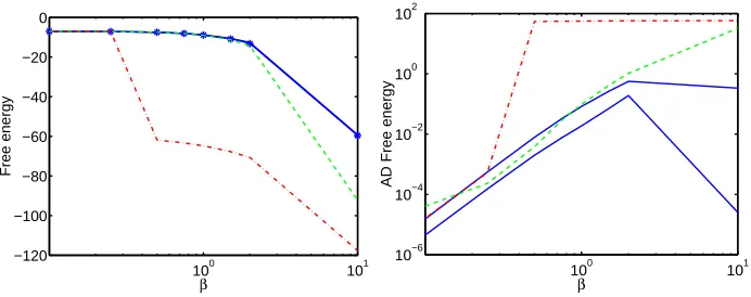
In figure 2 we compare estimates of the free energy. The results show that the simple factorized EC approach gives performance similar to (and in many case better than) the structured Bethe and Kikuchi approximations. The EC tree version is almost always better than the other approximations. The Kikuchi approximation is not uniquely defined, but depends upon the choice of “cluster-structure”. Different types of structures can give rise to quite different performance (Minka and Qi, 2004). The results given above is thus just to be taken as one realization of the Kikuchi method where the clusters are taken as all variable triplets. We expect the Kikuchi approximation to yield better results (probably better than EC in some cases) for an appropriate choice of sub-graphs, for example triangles forming a star for fully connected models and all squares for grids (Yedidia et al., 2001; Minka and Qi, 2004). EC can also be improved beyond trees as discussed in the Conclusion.
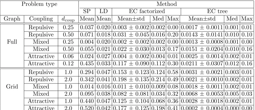
The second test is the set-up proposed by Wainwright and Jordan (2003, 2005). The N = 16 nodes are either fully connected or connected to nearest neighbors in a 4-by-4 grid. The external field (observation) strengths θi are drawn from a uniform distribution
θi ∼ U[−dobs, dobs] with dobs = 0.25. Three types of coupling strength statistics are con-sidered: repulsive (anti-ferromagnetic) Jij ∼ U[−2dcoup,0], mixed Jij ∼ U[−dcoup,+dcoup] and attractive (ferromagnetic)Jij ∼ U[0,+2dcoup] withdcoup >0. We compute the average absolute deviation on the marginals:
AAD = 1 N
X
i
|p(xi = 1)−p(xi= 1|method)|
over 100 trials testing the following methods: SP = sum-product (aka loopy belief propaga-tion (BP) or Bethe approximapropaga-tion) and LD = log-determinant maximizapropaga-tion (Wainwright and Jordan, 2003, 2005), EC factorized and EC tree. Results for SP and LD are taken from Wainwright and Jordan (2003). Note that instances where SP failed to converge were excluded from the results. A fact that is likely to bias the results in favor of SP. The results are summarized in table 6. The Bethe approximation always gives inferior results compared to EC. This might be a bit surprising for the sparsely connected grids. LD is a robust method which however seems to be limited in it’s achievable precision. EC tree is uniformly superior to all other approaches. It would be interesting to compare to the Kikuchi approximation which is known to give good results on grids.
A few comments about complexity, speed and rates of convergence: Both EC algorithms are O(N3). For the N = 16 simulations typical wall clock times were 0.5 sec. for exact computation, half of that for the loop tree and one-tenth for the factorized single-loop. Convergence is defined to be when||hg(x)iq− hg(x)ir||2 is below 10−12. Double loop
algorithms typically were somewhat slower (1-2 sec.) because a lot of outer loop iterations were required. This indicates that the bound optimized in the inner loop is very conservative for these binary problems. For the easy problems (small dcoup) all approaches converged. For the harder problems the factorized EP-style algorithms typically converged in 80-90 % of the cases. A greedy single-loop variant of the sequential double-loop algorithm, where the outer loop update is performed after every inner loop update, converged more often without being much slower than the EP-style algorithm. We treated the grid as a fully connected system yielding a complexity ofO(N3). Exploiting the structure using message passing, one can reduce the complexity of inference, i.e. calculating the covariance on the links, toO(N2).
7. Conclusion and Outlook
We have introduced a novel method for approximate inference which tries to overcome lim-itations of previous approximations in dealing with the correlations of random variables. While we have demonstrated its accuracy in this paper only for a model with binary ele-ments, it can also be applied to models with continuous random variables or hybrid models with both discrete and continuous variables (i.e. cases where further approximations are needed in order to apply Bethe/Kikuchi approaches).
100 101 10−6
10−4 10−2 100
β
MAD 1 node marginals
100 101
10−5 10−4 10−3 10−2 10−1 100
MAD 2 node marginals
β
Figure 1: Maximal absolute deviation (MAD) for one- (left) and two-variable (right) marginals. EC factorized: upper full line (blue), EC tree: lower full line (blue), Bethe: dashed line (green) and Kikuchi: dash-dotted line (red).
100 101
−120 −100 −80 −60 −40 −20 0
Free energy
β 10
0
101 10−6
10−4 10−2 100 102
AD Free energy
β
Figure 2: Left plot: free energy exact: stars, EC factorized and tree: full lines virtually on top on each others (blue), Bethe: dashed line (green) and Kikuchi: dash-dotted (red). Right: Absolute devi-ation (AD) for the three approximdevi-ations, same line type (and color) as above. Lower full line is for the EC tree approxima-tion.
Problem type Method
SP LD EC factorized EC tree
Graph Coupling dcoup Mean Mean Mean±std Med Max Mean±std Med Max Repulsive 0.25 0.037 0.020 0.003±0.002 0.002 0.00 0.0017 ±0.0011 0.001 0.01 Repulsive 0.50 0.071 0.018 0.031±0.045 0.016 0.20 0.0143 ±0.0141 0.010 0.10 Full Mixed 0.25 0.004 0.020 0.002±0.002 0.002 0.00 0.0013 ±0.0008 0.001 0.00 Mixed 0.50 0.055 0.021 0.022±0.030 0.013 0.17 0.0151 ±0.0204 0.010 0.16 Attractive 0.06 0.024 0.027 0.004±0.002 0.004 0.01 0.0025 ±0.0014 0.002 0.01 Attractive 0.12 0.435 0.033 0.117±0.090 0.112 0.30 0.0211 ±0.0307 0.012 0.16 Repulsive 1.0 0.294 0.047 0.153±0.123 0.124 0.58 0.0031 ±0.0021 0.003 0.01 Repulsive 2.0 0.342 0.041 0.198±0.135 0.214 0.49 0.0021 ±0.0010 0.002 0.01 Grid Mixed 1.0 0.014 0.016 0.011±0.010 0.009 0.08 0.0018 ±0.0011 0.002 0.01 Mixed 2.0 0.095 0.038 0.082±0.081 0.034 0.32 0.0068 ±0.0053 0.005 0.03 Attractive 1.0 0.440 0.047 0.125±0.104 0.068 0.36 0.0028 ±0.0018 0.002 0.01 Attractive 2.0 0.520 0.042 0.177±0.125 0.198 0.41 0.0002 ±0.0004 0.000 0.00
Table 1: The average one-norm error on marginals for the Wainwright-Jordan set-up.
the complexity of the most computationally expensive part of the inference—calculating the moments of the Gaussian part—unchanged.
A generalization of our method to treat graphical models beyond pair-wise interaction may be obtained by iterating the approximation. This is useful in cases, where an initial three term approximation −lnZEC = −lnZ
q−lnZr + lnZs still contains non-tractable
component free energies. These individual terms can be further approximated using the EC approach. We can show that in such a way a variety of other relevant types of graph-ical models beyond the pair-wise interaction case (on certain directed graphs and mixture models) become tractable with our method.
For practical applicability of approximate inference techniques improvements in the nu-merical implementation of the free energy minimization are crucial. In the simulations in this paper we used both single and double loop algorithms. The single loop algorithms often converged very fast, i.e. inO(10) iterations to achieve a solution close to the machine precision. However, whether convergence could be achieved was instance dependent and depended upon set-up details like parallel/sequential update and damping factor. It seems that there is a lot of room for improvement here and theoretical analysis of convergence properties of algorithms will be important in this respect (Heskes and Zoeter, 2002). In the guaranteed convergent double loop approaches the free energy minimization is formulated in terms of a sequence of convex optimization problems. This allows for the application of theoretically well-founded and powerful techniques of convex optimization (Boyd and Vandenberghe, 2004). Unfortunately, for the problems considered here, convergence is typ-ically quite slow because we have to solve large number of the convex problems. This again underlines the need for further algorithmic development.
it is a signal that the approximation is breaking down. Another possible improvement could come from physics of disordered system where methods have be devised to analyze non-ergodic free energy landscapes (M´ezard et al., 1987). This will allow to make improved estimates of the free energy and marginals for example binary variables with large coupling strengths.
Acknowledgments
Discussions with and suggestions by Kees Albers, Bert Kappen, Tom Minka, Wim Wiegerinck, Onno Zoeter and anonymous referees are greatly appreciated. Special thanks to Wim for his contributions to clarifying the single loop algorithm concepts.
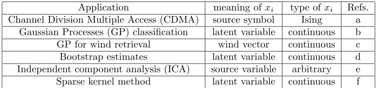
Appendix A. Applications
In this appendix we give list of of previous applications of the ADATAP method which is a special case of the EC approach to models with the factorization eqs. (6) and (7).
Application meaning ofxi type ofxi Refs.
Channel Division Multiple Access (CDMA) source symbol Ising a Gaussian Processes (GP) classification latent variable continuous b
GP for wind retrieval wind vector continuous c
Bootstrap estimates latent variable continuous d Independent component analysis (ICA) source variable arbitrary e Sparse kernel method latent variable continuous f
Table 2: Examples of applications of simplest version of EC, ADATAP. The references are a: Fabricius and Winther (2004), b: Opper and Winther (1999, 2000); Minka (2001a,b), c: Cornford et al. (2004), d: Malzahn and Opper (2003, 2004), e: Hojen-Sorensen et al. (2002) and f: Qui˜nonero-Candela and Winther (2003).
Appendix B. Dual Formulation
In this appendix we present an alternative route to EC free energy approximation using a two stage variational formulation. The result is the so-called Gibbs free energy which is the Lagragian dual of the Helmholtz free energy eq. (19).
B.1 Gibbs Free Energies and Two Stage Inference
In this framework, one starts with the well known fact that the true, intractable distribution p(x) = f(Zx) is implicitly characterized as the solution of an optimization problem defined through the relative entropy or KL divergence
KL(q, p) = Z
dxq(x) lnq(x)
betweenpand other trial or approximate distributionsq. We introduce the Gibbs free energy (GFE) approach, (see, e.g. Roepstorff, 1994; Csat´o et al., 2002; Wainwright and Jordan, 2003, 2005) which splits this optimization into a two stage process. One first constrains the trial distributions q by fixing the values of the generalized momentshg(x)iq. We define the
Gibbs free energyG(µµµ) as
G(µµµ) = min
q {KL(q, p)| hg(x)iq=µµµ} −lnZ . (39)
The term lnZ has been subtracted to make the resulting expression independent of the intractable partition function Z.
In a second step, the moments of the distribution and also the partition functionZ are found within the same approach by relaxing the constraints and further minimizing G(µµµ) with respect to theµµµ.
min
µ
µµ G(µµµ) = −lnZ (40)
hg(x)i = argmin
µ µ
µ G(µµµ) . (41)
A variational bound approximation is recovered by restricting the minimization in eq. (39) to a tractable family of densities q. Note that the values for µµµ in the definition of G(µµµ) cannot be chosen arbitrarily. For a detailed discussion of this problem, see Wainwright and Jordan (2003, 2005). We will not discuss these constraints here, but leave this, when necessary, to the discussion of concrete models.
Gibbs free energy and duality. The optimization problem eq. (39) is solved by the density given by
q(x) = f(x)
Z(λ)exp λ
Tg(x)
. (42)
λ = λ(µµµ) is the vector of Lagrange parameters chosen such that the moment conditions
hg(x)iq=µµµare fulfilled, i.e. λsatisfies
∂lnZ(λ)
∂λ =µµµ . (43)
In the following, it should be clear from the context when λ is a free variable or is to be determined from eq. (43). Inserting the optimizing distribution eq. (42) into the definition of the Gibbs free energy eq. (39), we get the simpler expression:
G(µµµ) =−lnZ(λ(µµµ)) +λT(µµµ)µµµ= max
λ
−lnZ(λ) +λTµµµ . (44)
showing that G(µµµ) is the Lagrangian dual of lnZ(λ).
Derivatives with respect to parameters. We will use the following result about the derivative of G with respect to a parameter t in the density. Using the notation p(x|t) = f(Zx,t)
t (which should not be confused with a conditional probability), we
calcu-late the derivative of G(µµµ, t) using (43) and (44) as for fixedµµµ: dG(µµµ, t)
dt = −
∂lnZ(λ, t)
∂t +
µ µ
µ−∂lnZ(λ, t) ∂λ
dλT
dt =−
∂lnZ(λ, t)
∂t , (45)
whereZ(λ, t) =R
B.2 An Interpolation Representation of Free Energies
If the densityp factors into a tractable fq and an intractable part fr, according to eq. (2),
we can construct a representation of the Gibbs free energy which also separates into two corresponding parts. This is done by treating fr(x) as a perturbation which is smoothly
turned on using a parameter 0 ≤ t ≤ 1. We define fr(x, t) to be a smooth interpolation
between the trivial fr(x, t = 0) = 1 and the “full” intractable fr(x, t = 1) = fr(x). The
most common choice is to setfr(x, t) = [fr(x)]t, but a more complicated construction can be
necessary, whenfrcontainsδ-distributions, see appendix E. However, we will see later, that
an explicit construction of the interpolation will not be necessary for our approximation. Next, we define the interpolating density and the associated optimizing distribution for the Gibbs free energy
p(x|t) = 1 Zt
fq(x)fr(x, t) (46)
q(x|t) = 1 Zq(λ, t)
fq(x)fr(x, t) exp λTg(x)
, (47)
where
Zq(λ, t) =
Z
dxfq(x)fr(x, t) exp λTg(x)
(48)
and the corresponding free energyGq(µµµ, t) = maxλ
−lnZq(λ, t) +λTµµµ . For later
conve-nience, we have given a subscript toGand lnZto indicate which approximating distribution is being used. We can now use the following simple identity for the free energyG(µµµ, t)
G(µµµ,1)−G(µµµ,0) = Z 1
0
dtdG(µµµ, t)
dt (49)
to relate the Gibbs free energy of the intractable model G(µµµ) = G(µµµ, t = 1) and tractable model G(µµµ, t= 0). Using eq. (20), we get
dG(µµµ, t)
dt =−
∂lnZ(λ, t)
∂t =−
dlnfr(x, t)
dt
q(x|t)
. (50)
While this representation can be used to re-derive a variational bound approximation (see Appendix F), we will next re-derive a dual representation of the EC free energy by making an approximation similar in spirit to the one used in Section 3. We again assume that besides the family of distributions eq. (4), there is a second family which can be used as an approximation to the distribution eq. (46). It is defined by
r(x|t) = 1 Zr(λ, t)
fr(x, t) exp λTg(x) , (51)
where, as before the parametersλare chosen in such a way as to guaranteeconsistency for the expectationsof g, i.e. hg(x)ir(x|t)=µµµand
Zr(λ, t) =
Z
dxfr(x, t) exp λTg(x)
Obviously,r(x|t) defines another Gibbs free energy which in its dual representation eq. (44) is given by
Gr(µµµ, t) = max λ
−lnZr(λ, t) +λTµµµ . (53)
Using the density r(x|t) to treat the integral in eq. (49), we make the approximation Z 1
0 dt
dlnfr(x, t)
dt
q(x|t) ≈
Z 1 0
dt
dlnfr(x, t)
dt
r(x|t)
. (54)
The fact that both types of densities eqs. (47) and (51) contain the same exponential factor fr(x, t) exp λTg(x) allows us to carry out the integral over the interaction strength t on
the right hand side of eq. (54) in closed form without specifying the interpolating term fr(x, t) explicitly. We simply use the relations eqs. (49) and (50) again, but this time for
the free energy eq. (53) to get Z 1
0 dt
dlnfr(x, t)
dt
r(x|t)
=Gr(µµµ,1)−Gr(µµµ,0). (55)
Using the approximation eq. (54) and the two exact relation eqs. (49) forq andr we arrive at theexpectation consistent (EC)approximation:
Gq(µµµ,1)≈Gq(µµµ,0) +Gr(µµ,µ 1)−Gr(µµµ,0)≡GEC(µµµ) . (56)
Recovering the EC free energy eq. (19) Using the duality expression for the free energies eq. (44), the free energy approximation can be written as
GEC(µµµ) = Gq(µµµ) +Gr(µµµ)−Gs(µµµ) (57)
= max
λq,λr
min
λs
−lnZq(λq)−lnZr(λr) + lnZs(λs) +µµµT(λq+λr−λs) ,
where we have defined Gq(µµµ) = Gq(µµµ,0), Gr(µµµ) = Gr(µµµ,1) and Gs(µµµ) = Gr(µµµ,0). To
obtain the corresponding approximation for the Helmholtz free energy −lnZ, we should minimize this expression with respect toµµµ. Any local minimum will be characterized by the vanishing of the partial derivative with respect to µµµ. This yields the following constraint on the Lagrange parameters
λq+λr−λs= 0 , (58)
which can be used to eliminate, sayλr and we recover eq. (19).
such an algorithm first upper bounds the concave function −Gs(µµµ) by the linear function
−(µµµ−µµµ(t))T ∂Gs(µµµ)
∂µµµ
µµµ=µµµ(t).
In terms of the corresponding Lagrange-parameter λs(t) = ∂G∂µsµµ(µµµ)
µ
µµ=µµµ(t), this yields GEC(µµµ) ≤ Gq(µµµ) +Gr(µµµ)−(µµµ−µµµ(t))T λs(t)
= max
λq,λr
−lnZq(λq)−lnZr(λr) +µµµT(λq+λr) + lnZs(λs(t)) ≡GECt (µµµ)
Minimizing GECt (µµµ) with respect toµµµ, we immediately get min
µ µµ G
EC
t (µµµ) = max λq
{−lnZq(λq)−lnZr(λs−λq)}+ lnZs(λs(t)) =F(λs(t)), (59)
whereF(λs(t)) was introduced in eq. (26). The new approximation is computed as
µ µ
µ(t+ 1) =hg(x)iq(t+1) .
Hence, this double loop procedure is equivalent to the one defined in Section 5, demon-strating that the sequenceF(λs(t)) yields nondecreasing upper bounds to the minimal EC
Gibbs free energy.
Appendix C. Tree-Connected Graphs
For the EC tree approximation we will need to make inference on tree-connected graphs. To handle a problem with binary variables both binary and Gaussian distributed variables on a tree will be needed. We will write the model as
p(x) = 1 Z
Y
i
ψi(xi) exp
−1
2x
TΛx+γTx
,
where ψi(xi) = δ(xi −1) +δ(xi+ 1) for binary and ψi(xi) = 1 for Gaussian. Assuming
that Λdefines a tree one can express the free energy in terms of single- and two-node free energies (Yedidia et al., 2001):
−lnZ(λ) =− X (ij)∈G
lnZij(λ(ij))−
X
i
(1−ni) lnZi(λ(i)) , (60)
whereλ(ij)=γi(ij), γj(ij),Λ(iiij),Λij(ij),Λ(jjij)are the parameters associated with the moments g(ij) =
xi, xj,−x
2
i
2 ,−xixj,−
x2
j
2
and ni is the number of links to node i. The two-node
partition functionZij is given by
Zij(λ(ij)) =
Z
dxidxjψi(xi)ψj(xj)eγixi+γjxj−Λijxixj−Λiix
2
i/2−Λjjx2j/2 . (61)
The Gibbs free energy G(µµµ) = maxλ{−lnZ(λ) +λTµµµ}can be written in terms of one-and two-node Gibbs free energies:
G(µµµ) = X (ij)∈G
lnGij(µµµ(ij))−
X
i
(1−ni)Gi(µµµ(i))
Gij(µµµ(ij)) = max
λ(ij){−lnZij(λ
(ij)) + (λ(ij))Tµµµ(ij)
} , (62)
whereµµµ(ij)=hg(ij)(x)i. We can writeλ=P
(ij)∈Gλ(ij)− P
i(1−ni)λ(i), where λ(ij) here
should be understood as a vector of the same length as g having non-zero elements for moments defined for the pair (ij). By solving the max condition we can write the Lagrange parameters in terms of the mean values mi = hxii and covariances χij = hxixji −mimj.
This will be useful when we derive algorithms for optimizing the free energy in section 5 where we need to solve for λin terms ofµµµ. For binary variables we get:
γi(i) = tanh−1(mi)
γi(ij) = 1 2tanh
−1
mi+mj
1 +hxixji
+ 1
2tanh −1
mi−mj
1− hxixji
γj(ij) = 1 2tanh
−1
mi+mj
1 +hxixji
+ 1
2tanh −1
mj −mi
1− hxixji
Λ(ijij) = −1 2tanh
−1
hxixji+mi
1 +mj
− 12tanh−1
hxixji −mi
1−mj
and for Gaussian definingm(ij)=
mi
mj
and χ(ij) ≡
χii χij
χji χjj
:
γ(ii) = mi/χii and Λ(ii) = 1/χii γ(ij) = (χ(ij))−1m(ij) and Λ(ij) = (χ(ij))−1 .
Finally, we will also need to make inference about the mean values and covariances on the tree for the binary variables. This can be done effectively by message passing on the tree. The message from link (ij) to node i denoted by r(ij)→i can be obtained by the following recursion (MacKay, 2003)
r(ij)→i = tanh(−Λij) tanh(θj\i)
θj\i = θj+
X
k,(jk)∈G,(jk)6=(ij)
r(jk)→j .
The recursion converges in one collect and one distribute messages sweep (to/from an ar-bitrarily chosen root node). Inference is linear because the tree contains N −1 links. The mean values and correlations are given by
mi = tanh
θi+
X
j,(ij)∈G
r(ij)→i
hxixji =
e−Λijcosh(θ
i\j+θj\i)−eΛijcosh(θi\j−θj\i)
e−Λijcosh(θ
i\j+θj\i) +eΛijcosh(θi\j−θj\i)
Appendix D. Single Loop Algorithmic Recipes
In this appendix we give the algorithmic recipes for one sequential algorithm for the factor-ized EC and a parallel algorithm for tree EC. The sequential algorithm is close in spirit to Expectation Propagation withψi(xi) and exp γr,ixi−12Λr,ix2i
being what is called exact and approximate factors, respectively (Minka, 2001b):
• Initialize mean and covariance ofr-distribution:
mr := (Λr−J)−1(γr+θ) χr := (Λr−J)−1
withγr=0and Λr set such that the covariance is positive definite.
Run sequentially over the nodes: 1. Send message from r toqi
• Calculate separator si: γs,i:=mr,i/χr,ii and Λs,i:= 1/χr,ii.
• Updateqi: γq,i:=γs,i−γr,i and Λq,i:= Λs,i−Λr,i.
• Update moments ofqi: mq,i:= tanh(γq,i) and χq,ii = 1−m2q,i.
2. Send message from qi tor
• Calculate separator si: γs,i:=mq,i/χq,ii and Λs,i:= 1/χq,ii.
• Updater: γr,i :=γs,i−γq,i, ∆Λr,i:= Λs,i−Λq,i−Λr,i and Λr,i:= Λs,i−Λq,i.
• Update moments ofr (see eq. 37):
χr := χr− ∆Λr,i
1 + ∆Λr,i[χr]ii
[χr]i[χr]Ti
mr := χr(γr+θ) .
Convergence is reached when and if mr=mq and χr,ii =χq,ii,i= 1, . . . , N. The
compu-tational complexity of the algorithm is O(N3Nite) because each Sherman-Morrison update isO(N2) and we make N of those in each sweep over the nodes.
The tree EC algorithm is very similar. The only difference is that it is parallel and uses inference on a tree graph, see appendix C for details on the tree inference:
• Initialize as above. Update:
1. Send message from r toq
• Calculate separator s: [γs,Λs] := Lagrange Gauss tree(mr,tree(χr)), where
tree() sets all non-tree elements to zero.
• Updateq: γq :=γs−γr and Λq:=Λs−Λr.
• Update moments ofq: [mq,χq] := inference binary tree(γq,Λq) will only return
2. Send message from q tor
• Calculate separator s: [γs,Λs] := Lagrange Gauss tree(mq,χq).
• Updater: γr :=γs−γq and Λr:=Λs−Λq.
• Update moments ofr: χr:= (Λr−J)−1 and mr :=χr(γr+θ).
Convergence is reached whenmq =mrandχq= tree(χr). This algorithm is alsoO(N3Nite) because of the matrix inverse. All other operations are O(N) even though these will dom-inate for small N. Typically when convergent both algorithms converge in Nite = O(10) steps.
Appendix E. Interpolation Scheme for Discrete Variables
The Ising case eq. (9) can be treated by defining the bimodal density
fr(x, t) = N
Y
i=1
exph−1−tt(x4
i −2x2i)
i
√
1−t
which interpolates between a constant function for t= 0 and becomes proportional to the Dirac measures eq. (9) in the limit t → 1. Other discrete variables can be treated in a similar fashion.
Appendix F. Re-deriving the Variational Bound Approximation
The choicefr(x, t) =tlnfr(x) for the interpolation can be used for a perturbation expansion
of the free energy G(µµµ, t) in powers of t, where at the end one sets t = 1. The lowest nontrivial (first) order term is obtained by replacing q(x|t) by q(x|0) in eq. (50). In this case, one obtains an approximation to the Gibbs free energy given by
G(µµµ)≈G(µµµ,0)− Z 1
0 dt
dlnfr(x, t)
dt
q(x|0)
=G(µµµ,0)− hlnfr(x)iq(x|0) . (63)
For the second order term of this so-called Plefka expansion see, e.g. Plefka (1982) and several contributions in Opper and Saad (2001).
For comparison, we define a variational bound approximation, where the minimization in eq. (39) is restricted to the familyF of densities of the form eq. (4), i.e.
Gvar(µµµ) = min
q∈F{KL(q, p)| hg(x)iq=µµµ} −lnZ . (64)
References
H. Attias. A variational Bayesian framework for graphical models. In T. Leen, T. G. Dietterich, and V. Tresp, editors, Advances in Neural Information Processing Systems 12, pages 209–215. MIT Press, 2000.
C. M. Bishop, D. Spiegelhalter, and J. Winn. Vibes: A variational inference engine for Bayesian networks. In S. Becker, S. Thrun, and K. Obermayer, editors, Advances in Neural Information Processing Systems 15, pages 777–784. MIT Press, 2003.
S. Boyd and L. Vandenberghe. Convex Optimization. Cambridge University Press, 2004. D. Cornford, L. Csat´o, D. J. Evans, and M. Opper. Bayesian analysis of the scatterometer
wind retrieval inverse problem: Some new approaches. Journal Royal Statistical Society B, 66:1–17, 2004.
L. Csat´o, M. Opper, and O. Winther. TAP Gibbs free energy, belief propagation and sparsity. In T. G. Dietterich, S. Becker, and Z. Ghahramani, editors,Advances in Neural Information Processing Systems 14, pages 657–663, Cambridge, MA, 2002. MIT Press. T. Fabricius and O. Winther. Correcting the bias of subtractive interference cancellation
in cdma: Advanced mean field theory. Submitted to IEEE trans. Inf. Theory, 2004. T. Heskes, K. Albers, and H. Kappen. Approximate inference and constrained optimization.
In Proceedings UAI-2003, pages 313–320. Morgan Kaufmann, 2003.
T. Heskes and O. Zoeter. Expectation propagation for approximate inference in dynamic Bayesian networks. In A. Darwiche and N. Friedman, editors, Proceedings UAI-2002, pages 216–233, 2002.
P. A.d.F.R. Hojen-Sorensen, O. Winther, and L. K. Hansen. Mean field approaches to independent component analysis. Neural Computation, 14:889–918, 2002.
Michael I. Jordan, Zoubin Ghahramani, Tommi S. Jaakkola, and Lawrence K. Saul. An introduction to variational methods for graphical models. Mach. Learn., 37:183–233, 1999.
D. J. C. MacKay. Information Theory, Inference, and Learning Algorithms. Cambridge University Press, 2003.
D. Malzahn and M. Opper. An approximate analytical approach to resampling averages.
Journal of Machine Learning Research, pages 1151–1173, 2003.
D. Malzahn and M. Opper. Approximate analytical bootstrap averages for support vector classifiers. In Sebastian Thrun, Lawrence Saul, and Bernhard Sch¨olkopf, editors,Advances in Neural Information Processing Systems 16. MIT Press, 2004.
M. M´ezard, G. Parisi, and M. A. Virasoro. Spin Glass Theory and Beyond, volume 9 of
T. P. Minka. Expectation propagation for approximate Bayesian inference. In J. S. Breese and D. Koller, editors, Proceedings UAI-2001, pages 362–369. Morgan Kaufmann, 2001a. T. P. Minka. A family of algorithms for approximate Bayesian inference. PhD thesis, MIT
Media Lab, 2001b.
T. P. Minka and Y. Qi. Tree-structured approximations by expectation propagation. In S. Thrun, L. Saul, and B. Sch¨olkopf, editors,Advances in Neural Information Processing Systems 16. MIT Press, 2004.
M. Opper and D. Saad, editors. Advanced Mean Field Methods: Theory and Practice. MIT Press, 2001.
M. Opper and O. Winther. Mean field methods for classification with gaussian processes. In M. S. Kearns, S. A. Solla, and D. A. Cohn, editors, Advances in Neural Information Processing Systems 11, pages 309–315. MIT Press, 1999.
M. Opper and O. Winther. Gaussian processes for classification: Mean field algorithms.
Neural Computation, 12:2655–2684, 2000.
M. Opper and O. Winther. Adaptive and self-averaging Thouless-Anderson-Palmer mean field theory for probabilistic modeling. Phys. Rev. E, 64:056131, 2001a.
M. Opper and O. Winther. Tractable approximations for probabilistic models: The adaptive Thouless-Anderson-Palmer mean field approach. Phys. Rev. Lett., 86:3695, 2001b. M. Opper and O. Winther. Variational linear response. In S. Thrun, L. Saul, and
B. Sch¨olkopf, editors,Advances in Neural Information Processing Systems 16. MIT Press, Cambridge, MA, 2004.
T. Plefka. Convergence condition of the TAP equation for the infinite-range Ising spin glass.
J. Phys. A, 15:1971, 1982.
J. Qui˜nonero-Candela and O. Winther. Incremental gaussian processes. In S. Thrun S. Becker and K. Obermayer, editors,Advances in Neural Information Processing Systems 15, pages 1001–1008. MIT Press, 2003.
G. Roepstorff. Path Integral Approach to Quantum Physics, An Introduction. Springer -Verlag Berlin Heidelberg, New York, 1994.
M. Suzuki, editor. Coherent Anomaly Method, Mean Field, Fluctuations and Symmetries. World Scientific, 1995.
L. Vandenberghe, S. Boyd, and S.-P Wu. Determinant maximization with linear matrix inequality constraints. SIAM Journal on Matrix Analysis and Applications, 19:499–533, 1998.
M. J. Wainwright and M. I. Jordan. A variational principle for graphical models. In S. Haykin, J. Principe, S. Sejnowski, and J McWhirter, editors, New Directions in Sta-tistical Signal Processing: From Systems to Brain. MIT Press, 2005.
M. Welling and Y.W. Teh. Approximate inference in Boltzmann machines. Artificial Intel-ligence, 143:19–50, 2003.
J. S. Yedidia, W. T. Freeman, and Y. Weiss. Generalized belief propagation. In T. K. Leen, T. G. Dietterich, and V. Tresp, editors,Advances in Neural Information Processing Systems 13, pages 689–695, 2001.
A. L. Yuille. CCCP algorithms to minimize the Bethe and Kikuchi free energies: convergent alternatives to belief propagation. Neural Computation, 14:1691–1722, 2002.