Mixed Membership Stochastic Blockmodels

Mixed Membership Stochastic Blockmodels

Edoardo M. Airoldi∗ [email protected]

David M. Blei [email protected]

Department of Computer Science Princeton University

Princeton, NJ 08544, USA

Stephen E. Fienberg† [email protected]

Department of Statistics Carnegie Mellon University Pittsburgh, PA 15213, USA

Eric P. Xing [email protected]

School of Computer Science Carnegie Mellon University Pittsburgh, PA 15213, USA

Editor: Tommi Jaakkola

Abstract

Consider data consisting of pairwise measurements, such as presence or absence of links between pairs of objects. These data arise, for instance, in the analysis of protein interactions and gene regulatory networks, collections of author-recipient email, and social networks. Analyzing pair-wise measurements with probabilistic models requires special assumptions, since the usual inde-pendence or exchangeability assumptions no longer hold. Here we introduce a class of variance allocation models for pairwise measurements: mixed membership stochastic blockmodels. These models combine global parameters that instantiate dense patches of connectivity (blockmodel) with local parameters that instantiate node-specific variability in the connections (mixed membership). We develop a general variational inference algorithm for fast approximate posterior inference. We demonstrate the advantages of mixed membership stochastic blockmodels with applications to so-cial networks and protein interaction networks.

Keywords: hierarchical Bayes, latent variables, mean-field approximation, statistical network analysis, social networks, protein interaction networks

1. Introduction

The problem of modeling relational information among objects, such as pairwise relations repre-sented as graphs, arises in a number of settings in machine learning. For example, scientific litera-ture connects papers by citations, the Web connects pages by links, and protein-protein interaction data connects proteins by physical binding records. In these settings, we often wish to infer hidden attributes of the objects from the observed measurements on pairwise properties. For example, we might want to compute a clustering of the web-pages, predict the functions of a protein, or assess

∗. Also in the Lewis-Sigler Institute for Integrative Genomics. Address correspondence to 228 Carl Icahn Laboratory, Princeton University.

the degree of relevance of a scientific abstract to a scholar’s query. Unlike traditional data collected from individual objects, relational data violate the classical independence or exchangeability as-sumptions made in machine learning and statistics. The observations are dependent because of the way they are connected. This interdependence suggests that a different set of assumptions is more appropriate.

There is a history of research devoted to analyzing relational data. One well-studied problem is clustering, grouping the objects to uncover a structure based on the observed patterns of interactions. Standard model-based clustering methods, for example, mixture models, are not immediately ap-plicable to relational data because they assume that the objects are conditionally independent given their cluster assignments. Rather, the latent stochastic blockmodel (Wang and Wong, 1987; Snijders and Nowicki, 1997) is an adaptation of mixture modeling to relational data. In that model, each ob-ject belongs to a cluster and the relationships between obob-jects are governed by the corresponding pair of clusters. With posterior inference, one identifies a set of latent roles which govern the ob-jects relationships with each other. A recent extension of this model relaxed the finite-cardinality assumption on the latent clusters with a nonparametric hierarchical Bayesian model based on the Dirichlet process prior (Kemp et al., 2004, 2006; Xu et al., 2006).

The latent stochastic blockmodel suffers from a limitation that each object can only belong to one cluster, or in other words, play a single latent role. However, many relational data sets are multi-facet. For example, when a protein or a social actor interacts with different partners, different functional or social contexts may apply and thus the protein or the actor may be acting according to different latent roles they can possible play. In this paper, we relax the assumption of single-latent-role for actors, and develop a mixed membership model for relational data. Mixed membership models, such as latent Dirichlet allocation (Blei et al., 2003), have re-emerged in recent years as a flexible modeling tool for data where the single cluster assumption is violated by the heterogeneity within of a data point. For almost two decades, these models have been successfully applied in many domains, such as surveys (Berkman et al., 1989; Erosheva, 2002), population genetics (Pritchard et al., 2000), document analysis (Minka and Lafferty, 2002; Blei et al., 2003; Buntine and Jakulin, 2006), image processing (Li and Perona, 2005), and transcriptional regulation (Airoldi et al., 2007).

The mixed membership model associates each unit of observation with multiple clusters rather than a single cluster, via a membership probability-like vector. The concurrent membership of a data in different clusters can capture its different aspects, such as different underlying topics for words constituting each document. This is also a natural idea for relational data, where the objects can bear multiple latent roles or cluster-memberships that influence their relationships to others. As we will demonstrate, a mixed membership approach to relational data lets us describe the interaction between objects playing multiple roles. For example, some of a protein’s interactions may be governed by one function; other interactions may be governed by another function.

. . . y11 21 31 N1 y y y . . . y12 22 32 N2 y y y . . . y13 23 33 N3 y y y . . . y1N 2N 3N NN y y y . . . . . . . . . . . . . . . B . . . 1 2 3 n

z11 y11

z11

z12 y12

z12

z13 y13

z13

z1N y1N

z1N

. . .

z21 y21

z21

z22 y22

z22

z23 y23

z23

z2N y2N

z2N

. . .

z

31 y31

z31

z

32 y32

z32

z

33 y33

z33

z

3N y3N

z3N

. . .

z

N 1 yN1

z

N 1

z

N2 yN2

z

N2

z

11 yN3

z

N3

z

NN yNN

z NN . . . . . . . . . . . . . . . . . . . . . 1 2 3 n B

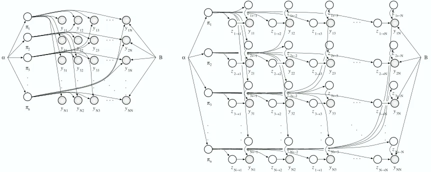
Figure 1: Two graphical model representations of the mixed membership stochastic blockmodel (MMB). Intuitively, the MMB summarized the variability of a graph with the blockmodel B and node-specific mixed membership vectors (left). In detail, a mixed membership,

πn(k), quantifies the expected proportion of times node n instantiates the connectivity pattern of group k, according to the blockmodel. In any given interaction, Y(n,m), how-ever, node n instantiates the connectivity pattern of a single group, zn→m(k). (right). We

did not draw all the arrows out of the block model B for clarity; all interactions depend on it.

In this paper, we develop mixed membership models for relational data.1 Models in this family include parameters to reduce bias due to sparsity, and can be used to analyze multiple collections of paired measurements, and collections of non-binary and multivariate paired measurements. We develop a fast nested variational inference algorithm that performs well in the relational setting and is parallelizable. We demonstrate the application of our technique to large-scale protein interaction networks and social networks. Our model captures the multiple roles that objects exhibit in interac-tion with others, and the relainterac-tionships between those roles in determining the observed interacinterac-tion matrix.

2. The Mixed Membership Stochastic Blockmodel

In this section, we describe the modeling assumptions if the mixed membership model of relational data. We represent observed relational data as a graph G= (

N

As a running example, we consider the monk data of Sampson (1968). Sampson measured a collection of sociometric relations among a group of monks by repeatedly asking questions such as “whom do you like?” and “whom do you dislike?” to determine asymmetric social relationships within the group. The questionnaire was repeated at four subsequent epochs. Information about these repeated, asymmetric relations was collapsed into a square binary table that encodes the di-rected connections between monks by Breiger et al. (1975). In analyzing this data, the goal is to determine the social structure within the monastery.

In the context of the monastery example, we assume K factions, that is, latent groups, exist in the monastery, and the observed network is generated according to distributions of group-membership for each monk and a matrix of group-group interaction strength. The per-monk distributions are specified by latent simplicial vectors. Each monk is associated with a randomly drawn vector~πi

for monk i, whereπi,gdenotes the probability of monk i belonging to group g. That is, each monk

can simultaneously belong to multiple groups with different degrees of affiliation strength. The probabilities of interactions between different groups are defined by a matrix of Bernoulli rates B_(K×K), where B(g,h)represents the probability of having a link between a monk from group g and a monk from group h.

For each monk, the indicator vector~zp→qdenotes the group membership of monk p when he

responds to survey questions about monk q and~zp←qdenotes the group membership of monk q when

he responds to survey questions about node p.2 N denotes the number of monks in the monastery, and recall that K denotes the number of distinct groups a monk can belong to.

More in general, monks can be represented by nodes in a graph, where directed (binary) edges represent positive responses to survey questions about a specific sociometric relation. In this abstract setting, the mixed membership stochastic blockmodel (MMB) posits that a graph G= (

N

• For each node p∈

N

– Draw a K dimensional mixed membership vector~πp∼Dirichlet(~α).

• For each pair of nodes(p,q)∈

N

N

– Draw membership indicator for the initiator,~zp→q ∼Multinomial(~πp).

– Draw membership indicator for the receiver,~zq→p ∼Multinomial(~πq).

– Sample the value of their interaction, Y(p,q)∼Bernoulli(~z_p>_→qB~zp←q).

1. In previous work we combined mixed membership and blockmodels to perform analyses of a single collection of bi-nary, paired measurements; namely, hypothesis testing, predicting and de-noising interactions within an unsupervised learning setting (Airoldi et al., 2005).

This process is illustrated as a graphical model in Figure 1. Note that the group membership of each node is context dependent. That is, each node may assume different membership when interacting to or being interacted by different peers. Statistically, each node is an admixture of group-specific interactions. The two sets of latent group indicators are denoted by{~zp→q: p,q∈

N

{~zp←q: p,q∈

N

Under the MMB, the joint probability of the data Y and the latent variables{~π1:N,Z→,Z←}can be written in the following factored form,

p(Y,~π1:N,Z→,Z←|~α,B) =

∏

p,q

P(Y(p,q)|~zp→q,~zp←q,B)P(~zp→q|~πp)P(~zp←q|~πq)

∏

P(~πp|~α). (1)

This model generalizes to two important cases. First, multiple networks among the same actors can be generated by the same latent vectors. This may be useful, for instance, to analyze multivariate sociometric relations. Second, in the MMB the data generating distribution is a Bernoulli, but B can be a matrix that parameterizes any kind of distribution. This may be useful, for instance, to analyze collections of paired measurements, Y , that take values in an arbitrary metric space. We elaborate on this in Section 5.

2.1 Modeling Sparsity

Adjacency matrices encoding binary pairwise measurements are often sparse, that is, they contain many zeros or non-interactions. It is useful to distinguish two sources of non-interaction: they may be the result of the rarity of interactions in general, or they may be an indication that the pair of relevant blocks rarely interact. In applications to social sciences, for instance, nodes may represent people and blocks may represent social communities. It is reasonable to expect that a large portion of the non-interactions is due to limited opportunities of contact between people rather than due to deliberate choices, the structure of which the blockmodel is trying to estimate. It is useful to account for these two sources of sparsity at the model level. A good estimate of the portion of zeros that should not be explained by the blockmodel B reduces the bias of the estimates of its elements.

Thus, we introduce a sparsity parameterρ∈[0,1]in the MMB to characterize the source of non-interaction. Instead of sampling a relation Y(p.q) directly the Bernoulli with parameter specified as above, we down-weight the probability of successful interaction to (1−ρ)·~z_p>_→qB~zp←q. This

is the result of assuming that the probability of a non-interaction comes from a mixture, 1−σpq= (1−ρ)·~z_p>_→q(1−B)~zp←q+ρ, where the weight ρcapture the portion zeros that should not be

explained by the blockmodel B. A large value ofρwill cause the interactions in the matrix to be weighted more than non-interactions, in determining plausible values for{~α,B,~π1:N}.

2.2 Summarizing and De-Noising Pairwise Measurements

It is useful to distinguish two types of data analysis that can be performed with the mixed-membership blockmodel. First, MMB can be used to summarize the data, Y , in terms of the global blockmodel, B, and the node-specific mixed memberships,Πs. Second, MMB can be used to de-noise the data, Y , in terms of the global blockmodel, B, and interaction-specific single memberships, Zs. In both cases the model depends on a small set of unknown constants to be estimated: α, and B. The like-lihood is the same in both cases, although, the rationale for including the set of latent variables Zs differs. When summarizing data, we could integrate out the Zs analytically; this leads to numerical optimization of a smaller set of variational parameters, Γs. We choose to keep the Zs to simplify inference. When de-noising, the Zs are instrumental in estimating posterior expectations of each interactions individually—a network analog to the Kalman Filter. The posterior expectations of an interaction is computed as follows, in the two cases,

E[Y(p,q) =1]≈~bπp0Bb~bπq and E[Y(p,q) =1]≈~bφ_p→q0Bb~bφ_p←q.

2.3 An Illustration: Crisis in a Cloister

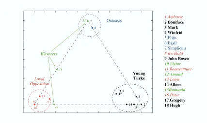
To illustrate the MMB, we return to an analysis of the monk data described above. Sampson (1968) surveyed 18 novice monks in a monastery and asked them to rank the other novices in terms of four sociometric relations: like/dislike, esteem, personal influence, and alignment with the monastic credo. We consider Breiger’s collation of Sampson’s data (Breiger et al., 1975). The original graph of monk-monk interaction is illustrated in Figure 2 (left).

Sampson spent several months in a monastery in New England, where novice monks were preparing to join a monastic order. Sampson’s original analysis was rooted in direct anthropological observations. He suggested the existence of tight factions among the novices: the loyal opposition (whose members joined the monastery first), the young turks (who joined later on), the outcasts (who were not accepted in the two main factions), and the waverers (who did not take sides). The events that took place during Sampson’s stay at the monastery supported his observations—members of the young turks resigned or were expelled over religious differences (John and Gregory). We shall

refer to the labels assigned by Sampson to the novices in the analysis below. For more analyses, we refer to Fienberg et al. (1985), Davis and Carley (2006) and Handcock et al. (2007).

Using the algorithms presented in Section 3, we fit the monks to MMB models for different numbers of groups, providing model estimates{αˆ,_Bˆ_{}and posterior mixed membership vectors}~πn

for each monk. Here, we use the following approximation to BIC to choose the number of groups in the MMB:

BIC=2·log p(Y)≈2·log p(Y|~bπ,Zb,~bα,Bb)− |~α,B| ·log|Y|,

which selects three groups, where|~α,B|is the number of hyper-parameters in the model, and|Y|is the number of positive relations observed (Volinsky and Raftery, 2000; Handcock et al., 2007). Note that this is the same number of groups that Sampson identified. We illustrate the fit of model fit via the predicted network in Figure 2 (Right). The three panels contrast the different resolution of the original adjacency matrix of whom-do-like sociometric relations (left panel) obtained in different uses of MMB. If the goal of the analysis if to find a parsimonious summary of the data, the amount of relational information that is captured by in ˆα,_{B, and}ˆ _E[~π|Y]leads to a coarse reconstruction of the original sociomatrix (central panel). If the goal of the analysis if to de-noising a collection of pairwise measurements, the amount of relational information that is revealed by ˆα,_Bˆ_,E[~π|Y]

andE[Z→,Z←|Y]leads to a finer reconstruction of the original sociomatrix, Y —relations in Y are re-weighted according to how much they make sense to the model (right panel).

1 2

3 4 5

6 7

8

9

10

11

12

13

14 15

16

17

18

Outcasts

Loyal

O pposition

Young Turks

Waverers

1 Ambrose

2 Boniface 3 M ark 4 W infrid 5 Elias 6 Basil 7 Simplicius 8 Berthold 9 John Bosco

10 Victor

11 Bonaventure

12 Amand

13 Louis 14 Albert

15Ramuald

16 Peter

17 Gregory

18 Hugh

Young Turks

Loyal Opposition

Outcasts

0.9

0.9 0.5

0.3 0.4

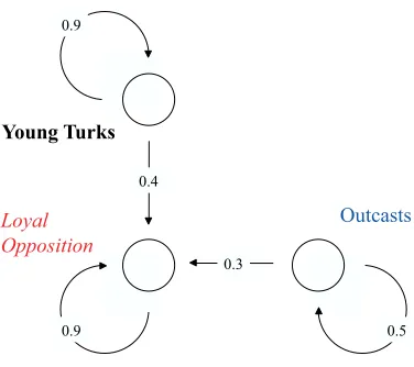
Figure 4: Estimated blockmodel in the monk data, ˆB.

The MMB provides interesting descriptive statistics about the actors in the observed graph. In Figure 3 we illustrate the the posterior means of the mixed membership scores,E[~π|Y], for the 18 monks in the monastery. Note that the monks cluster according to Sampson’s classification, with Young Turks, Loyal Opposition, and Outcasts dominating each corner respectively. We can see the central role played by John Bosco and Gregory, who exhibit relations in all three groups, as well as the uncertain affiliations of Ramuald and Victor. (Amand’s uncertain affiliation, however, is not captured.) The estimated blockmodel is shown in Figure 4.

3. Parameter Estimation and Posterior Inference

Two computational problems are central to the MMB: posterior inference of the per-node mixed membership vectors and per-pair roles, and parameter estimation of the Dirichlet parameters and Bernoulli rate matrix. We derive empirical Bayes estimates of the parameters(~α,B), and employ a mean-field approximation scheme for posterior inference.

3.1 Posterior Inference

The posterior inference problem is to compute the posterior distribution of the latent variables given a collection of observations. The normalizing constant of the posterior distribution is the marginal probability of the data, which requires an integral over the simplicial vectors~πp,

p(Y|~α,B) = Z

Π

∑

∏

P(Y(p,q)|~zp→q,~zp←q,B)P(~zp→q|~πp)P(~zp←q|~πq)

∏

P(~πp|~α)

!

d~π,

We appeal to variational methods (Jordan et al., 1999; Wainwright and Jordan, 2003). The main idea behind variational methods is to first posit a distribution of the latent variables with free parameters, and then fit those parameters such that the distribution is close in Kullback-Leibler divergence to the true posterior. The variational distribution is simpler than the true posterior so that the optimization problem can be approximately solved. Good reviews of variational methods can be found in Wainwright and Jordan (2003), Xing et al. (2003), Bishop et al. (2003) and Airoldi (2007). In the MMB, we begin by bounding the log of the marginal probability of the data with Jensen’s inequality,

log p(Y|α,B)≥Eq[log p(Y,~π1:N,Z→,Z←|α,B) ]−Eq[log q(~π1:N,Z→,Z←) ].

We have introduced a distribution of the latent variables q that depends on a set of free parameters. We specify q as the mean-field fully-factorized family,

q(~π_1:N,Z→,Z←|~γ1:N,Φ→,Φ←) =

∏

p

q1(~πp|~γp)

∏

p,q

q2(~zp→q|~φp→q)q2(~zp←q|~φp←q)

,

where q1 is a Dirichlet, q2 is a multinomial, and {~γ1:N,Φ→,Φ←} are the set of free variational

parameters that are optimized to tighten the bound.

Tightening the bound with respect to the variational parameters is equivalent to minimizing the KL divergence between q and the true posterior. When all the nodes in the graphical model are conjugate pairs or mixtures of conjugate pairs, we can directly write down a coordinate ascent algo-rithm for this optimization to reach a local maximum of the bound. The updates for the variational multinomial parameters are

ˆ

φp→q,g ∝ eEq[logπp,g]·

∏

B(g,h)Y(p,q)·(1−B(g,h) )1−Y(p,q)

φp←q,h

(2)

ˆ

φp←q,h ∝ eEq[logπq,h]·

∏

B(g,h)Y(p,q)·(1−B(g,h) )1−Y(p,q)

φp→q,g

, (3)

for g,h=1, . . . ,K. The update for the variational Dirichlet parametersγp,kis

ˆ

γp,k=αk+

∑

φp→q,k+

∑

φp←q,k, (4)

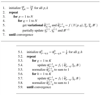
for all nodes p=1, . . . ,N and k=1, . . . ,K. The complete coordinate ascent algorithm is described in Figure 5.

To improve convergence, we employed a nested variational inference scheme based on an al-ternative schedule of updates to the traditional ordering. In a typical schedule for coordinate ascent (which we call “na¨ıve variational inference”), one initializes the variational Dirichlet parameters

~γ1:N and the variational multinomial parameters (~φp→q,~φp←q)to non-informative values, and then

iterates the following two steps until convergence: (i) update~φp→q andφp←q for all edges(p,q),

and (ii) update~γp for all nodes p∈

N

1. initialize~γ0

pk=

2N

K for all p,k

2. repeat

3. for p=1 to N

4. for q=1 to N

5. get variational~φt+_p→1_qand~φt+_p←1_q= f (Y(p,q),~γt

p,~γtq,Bt )

6. partially updateγ~t+p 1,γq~t+1and Bt+1

7. until convergence

5.1. initializeφ0_p→q,g=φ0

p←q,h=K1 for all g,h

5.2. repeat

5.3. for g=1 to K

5.4. updateφs+_p→1_q∝f1(~φsp←q,~γp,B)

5.5. normalize~φs+_p→1_qto sum to 1 5.6. for h=1 to K

5.7. updateφs+_p←1_q∝f2(~φsp→q,~γq,B)

5.8. normalize~φs+_p←1_qto sum to 1 5.9. until convergence

Figure 5: Top: The two-layered variational inference for (~γ,φp→q,g,φp←q,h)and M=1. The

in-ner algorithm consists of Step 5. The function f is described in details in the bottom panel. The partial updates in Step 6 for~γand B refer to Equation 4 of Section B.4 and Equation 5 of Section B.5, respectively. Bottom: Inference for the variational parame-ters(~φp→q,~φp←q)corresponding to the basic observation Y(p,q). This nested algorithm

details Step 5 in the top panel. The functions f1 and f2 are the updates forφp→q,g and φp←q,hdescribed in Equations 2 and 3 of Section B.4.

perspective, the na¨ıve variational EM algorithm instantiates a large coordinate ascent algorithm, where the parameters can be divided into blocks. Blocks are processed in a specific order, and the parameters within each block get all updated each time.3 At every new iteration the na¨ıve algorithm sets all the elements of~γt+1

1:N equal to the same constant. This dampens the likelihood by suddenly breaking the dependence between the estimates of parameters in~bγt_1:N and in ˆBt that was being inferred from the data during the previous iteration.

Instead, the nested variational inference algorithm maintains some of this dependence that is being inferred from the data across the various iterations. This is achieved mainly through a different

scheduling of the parameter updates in the various blocks. To a minor extent, the dependence is maintained by always keeping the block of free parameters,(~φp→q,~φp←q), optimized given the

other variational parameters. Note that these parameters are involved in the updates of parameters in~γ1:N and in B, thus providing us with a channel to maintain some of the dependence among them, that is, by keeping them at their optimal value given the data.

Furthermore, the nested algorithm has the advantage that it trades time for space thus allowing us to deal with large graphs; at each variational cycle we need to allocate NK+2K scalars only. The increased running time is partially offset by the fact that the algorithm can be parallelized and leads to empirically observed faster convergence rates.

An alternative strategy to perform inference is given by Monte Carlo Markov chain (e.g., see Griffiths and Steyvers, 2004; Kemp et al., 2004). While powerful in some settings, MCMC is impractical here. There are too many variables to sample. The proposed nested variational EM algorithm outperforms MCMC variations (i.e., blocked and collapsed Gibbs samplers) in terms of memory requirements and convergence rates.

3.2 Parameter Estimation

We compute the empirical Bayes estimates of the model hyper-parameters{~α,B}with a variational expectation-maximization (EM) algorithm. Alternatives to empirical Bayes have been proposed to fix the hyper-parameters and reduce the computation. The results, however, are not always sat-isfactory and often times cause of concern, since the inference is sensitive to the choice of the hyper-parameters (Joutard et al., 2007). Empirical Bayes, on the other hand, guides the posterior inference towards a region of the hyper-parameter space that is supported by the data.

Variational EM uses the lower bound in Equation 5 as a surrogate for the likelihood. To find a local optimum of the bound, we iterate between fitting the variational distribution q to approximate the posterior and maximizing the corresponding bound with respect to the parameters. The latter M-step is equivalent to finding the MLE using expected sufficient statistics under the variational distribution. We consider the maximization step for each parameter in turn.

A closed form solution for the approximate maximum likelihood estimate of~αdoes not exist (Minka, 2003). We use a linear-time Newton-Raphson method, where the gradient and Hessian are

∂

L

∂αk = N

ψ(

∑

αk)−ψ(αk)

+

∑

ψ(γp,k)−ψ(

∑

γp,k)

,

∂

L

= N

I(k1=k2)·ψ

0_(αk

1)−ψ

0₍

∑

k αk)

.

The approximate MLE of B is

ˆ

B(g,h) =∑p,qY(p,q)·φp→qgφp←qh (1−ρ)·∑p_,qφp→qgφp←qh

,

for every index pair(g,h)∈[1,K]×[1,K]. Finally, the approximate MLE of the sparsity parameter

ρis

ˆ

ρ=∑p,q(1−Y(p,q) )·(∑g,hφp→qgφp←qh) ∑p,q∑g,hφp→qgφp←qh

Alternatively, we can fixρprior to the analysis; the density of the interaction matrix is estimated with ˆd=∑p_,qY(p,q)/N2, and the sparsity parameter is set to ˜ρ= (1−dˆ). This latter estimator

attributes all the information in the non-interactions to the point mass, that is, to latent sources other than the block model B or the mixed membership vectors~π1:N. It does however provide a quick recipe to reduce the computational burden during exploratory analyses.4

Several model selection strategies are available for complex hierarchical models (Joutard et al., 2007). In our setting, model selection translates into the determination of a plausible value of the number of groups K. In the various analyses presented, we selected the optimal value of K according to two strategies. On large networks, we selected K corresponding to the highest averaged held-out likelihood in a cross-validation experiment. On small networks—where cross-validation cannot be expected to work well, as we discuss in Section 5—we selected K using an approximation to BIC.

4. Experiments and Results

We present a study of simulated data and applications to social and protein interaction networks. Simulations are performed in Section 4.1 to show that both mixed membership,~π1:N, and the latent block structure, B, can be recovered from data, when they exist, and that the nested variational inference algorithm is faster than the na¨ıve implementation while reaching the same peak in the likelihood—all other things being equal.

The application to a friendship network among students in Section 4.2 tests the model on a real data set where we expect a well-defined latent block structure to inform the observed connectivity patterns in the network. In this application, the blocks are interpretable in terms of grades. We compare our results with those that were recently obtained with a simple mixture of blocks (Doreian et al., 2007) and with a latent space model (Handcock et al., 2007) on the same data.

The application to a protein interaction network in Section 4.3 tests the model on a real data set where we expect a noisy, vague latent block structure to inform the observed connectivity patterns in the network to some degree. In this application, the blocks are interpretable in terms functional biological contexts. This application tests to what extent our model can reduce the dimensionality of the data, while revealing substantive information about the functionality of proteins that can be used to inform subsequent analyses.

4.1 Exploring Expected Model Behavior with Simulations

In developing the MMB and the corresponding computation, our hope is the the model can recover both the mixed membership of nodes to clusters and the latent block structure among clusters in situations where a block structure exists and the relations are measured with some error. To sub-stantiate this claim, we sampled graphs of 100,300,and 600 nodes from blockmodels with 4,10,

and 20 clusters, respectively, using the MMB. We used different values ofαto simulate a range of settings in terms of membership of nodes to clusters—from unique(α=0.05)to mixed(α=0.25).

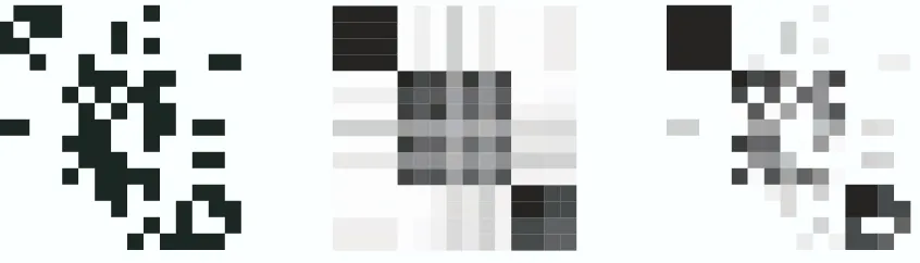
Recovering the truth. The variational EM algorithm successfully recovers both the latent block model B and the latent mixed membership vectors~π1:N. In Figure 6 we show the adjacency matri-ces of binary interactions where rows, that is, nodes, are reordered according to their most likely membership. The estimated reordering reveals the block model that was originally used to simulate

4. Note that ˜ρ=ρˆin the case of single membership. In fact, that impliesφmp→qg=φmp←qh=1 for some(g,h)pair, for

the interactions. Asαincreases, each node is likely to belong to more clusters. As a consequence, they express interaction patterns of clusters. This phenomenon reflects in the reordered interaction matrices as the block structure is less evident.

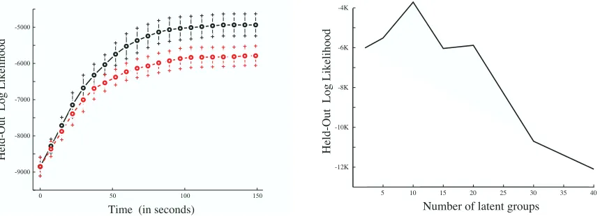
Nested variational inference. The nested variational algorithm drives the log-likelihood to con-verge faster to its peak than the na¨ıve algorithm. In Figure 7 (left panel) we compare the running times of the nested variational-EM algorithm versus the na¨ıve implementation. The nested algo-rithm, which is more efficient in terms of space, converged faster. Furthermore, the nested varia-tional algorithm can be parallelized given that the updates for each interaction(i,j)are independent of one another.

Choosing the number of blocks. The right panel of Figure 7 shows an example where cross-validation is sufficient to perform model selection for the MMB. The example shown corresponds to a network among 300 nodes with K=10 clusters. We measure the number of latent clusters

Figure 6: Adjacency matrices of corresponding to simulated interaction graphs with 100 nodes and 4 clusters, 300 nodes and 10 clusters, 600 nodes and 20 clusters (top to bottom) and

on the X axis and the average held-out log-likelihood, corresponding to five-fold cross-validation experiments, on the Y axis. The nested variational EM algorithm was xrun until convergence, for each value of K we tested, with a tolerance ofε=10−5. Our estimate for K occurs at the peak in the average held-out log-likelihood, and equals the correct number of clusters, K∗=10

4.2 Application to Social Network Analysis

We considered a friendship network among a group of 69 students in grades 7–12. The analysis here directly compares clustering results obtained by MMB to published clustering results obtained by competing models, in a setting where a fair amount of social segregation is expected (Doreian et al., 2007; Handcock et al., 2007).

The National Longitudinal Study of Adolescent Health is nationally representative study that explores the how social contexts such as families, friends, peers, schools, neighborhoods, and com-munities influence health and risk behaviors of adolescents, and their outcomes in young adulthood (Harris et al., 2003; Udry, 2003). As part of the survey, a questionnaire was administered to a sam-ple of students in each school, who were allowed to nominate up to 10 friends. We analyzed a friendship network among the students, at the same school that was considered by Handcock et al. (2007) and discussants. Friendship nominations were collected among 71 students in grades 7 to 12; two students did not nominate any friends. The network of binary, asymmetric friendship relations among the remaining 69 students that constitutes our data is shown in Figure 9 (left).

0 50 100 150

-9000 -8000 -7000 -6000 -5000

Time (in seconds)

H

el

d

-O

u

t

L

o

g

L

ik

el

ih

o

o

d

5 10 15 20 25 30 35 40

-12K -10K -8K -6K -4K

Number of latent groups

H

el

d

-O

u

t

L

o

g

L

ik

el

ih

o

o

d

Figure 8: The posterior mixed membership scores,~π, for the 69 students. Each panel correspond to a student; we order the clusters 1 to 6 on the X axis, and we measure the student’s grade of membership to these clusters on the Y axis.

Given the size of the network we used BIC to perform model selection, as in the monks example of Section 2.3. The results suggest a model with K∗=6 groups. (We fix K∗=6 in the analyses that follow.) The hyper-parameters estimated with the nested variational EM. They are ˆα=0.0487,

ˆ

ρ=0.936, and a fairly diagonal blockmodel,

ˆ B=

       

0.3235 0.0 0.0 0.0 0.0 0.0

0.0 0.3614 0.0002 0.0 0.0 0.0

0.0 0.0 0.2607 0.0 0.0 0.0002

0.0 0.0 0.0 0.3751 0.0009 0.0 0.0 0.0 0.0 0.0002 0.3795 0.0

0.0 0.0 0.0 0.0 0.0 0.3719

        .

tend to befriend other students in the same grade, with a few exceptions. The low degree of mixed membership explains the absence of obvious differences between the model-based reconstructions of the friendship relations with the two model variants (center and right).

Figure 9: Original matrix of friensdhip relations among 69 students in grades 7 to 12 (left), and friendship estimated relations obtained by thresholding the posterior expectations

~πp0_{B~πq|Y (center), and~φp}0_{B~φq|Y (right).}

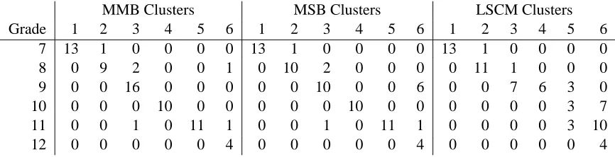
Next, we attempted a quantitative evaluation of the goodness of fit. In this data, the blocks are clearly interpretable a-posteriori in terms of grades. The mixed membership vectors provide a mapping between grades and blocks. Conditionally on such a mapping, we assign students to the grade they are most associated with, according to their posterior-mean mixed membership vectors, E[~πn|Y]. To be fair in the comparison with competing models, we assign students to a unique grade—despite MMB allows for mixed membership. Table 1 computes the correspondence of grades to blocks by quoting the number of students in each grade-block pair, for MMB versus the mixture blockmodel (MB) in Doreian et al. (2007), and the latent space cluster model (LSCM) in Handcock et al. (2007). The higher the sum of counts on diagonal elements is the better is the correspondence, while the higher the sum of counts off diagonal elements is the worse is the cor-respondence. MMB performs best by allocating 63 students to their grades, versus 57 of MB, and 37 of LSCM. Correspondence only partially captures goodness of fit, however, it is a good metric in the setting we consider, where a fair amount of clustering is present. The results suggest that the extra-flexibility MMB offers over MB and LSCM reduces bias in the prediction of the membership of students to blocks. In other words, mixed membership does not absorb noise in this example; rather it accommodates variability in the friendship relation that is instrumental in producing better predictions.

Concluding this example, we note how the model decouples the observed friendship patterns into two complementary sources of variability. On the one hand, the connectivity matrix B is a global, unconstrained set of hyper-parameters. On the other hand, the mixed membership vectors

~π_1:N provide a collection of node-specific latent vectors, which inform the directed connections in the graph in a symmetric fashion.

4.3 Application to Protein Interactions in Saccharomyces Cerevisiae

sug-MMB Clusters MSB Clusters LSCM Clusters

Grade 1 2 3 4 5 6 1 2 3 4 5 6 1 2 3 4 5 6

7 13 1 0 0 0 0 13 1 0 0 0 0 13 1 0 0 0 0

8 0 9 2 0 0 1 0 10 2 0 0 0 0 11 1 0 0 0

9 0 0 16 0 0 0 0 0 10 0 0 6 0 0 7 6 3 0

10 0 0 0 10 0 0 0 0 0 10 0 0 0 0 0 0 3 7

11 0 0 1 0 11 1 0 0 1 0 11 1 0 0 0 0 3 10

12 0 0 0 0 0 4 0 0 0 0 0 4 0 0 0 0 0 4

Table 1: Grade levels versus (highest) expected posterior membership for the 69 students, accord-ing to three alternative models. MMB is the proposed mixed membership stochastic block-model, MSB is a simpler stochastic block mixture model (Doreian et al., 2007), and LSCM is the latent space cluster model (Handcock et al., 2007).

gest different sets of interactions as reliable, we prefer the model that reveals functionally relevant interactions—as measured using the annotations.

Protein interactions (PPI) form the physical basis for the formation of stable protein complexes (i.e., protein clusters) and signaling pathways (i.e., cascades of protein interaction events) that carry out all major biological processes in the cell. A number of high-throughput experimental tech-nologies have been devised to determine the set of interacting proteins on a global scale in yeast. These include two-hybrid (Y2H) screens and mass spectrometry methods (Gavin et al., 2002; Ho et al., 2002; Krogan et al., 2006). High-throughput technologies, however, often miss to identify interactions that are not present under the given conditions. Specific wet-lab methods employed by a certain technology, such as tagging, may disturb the formation of a stable protein complex, and weakly associated components may dissociate and escape detection. Statistical models that encode information about functional processes with high precision are an essential tool for carrying out probabilistic de-noising of biological signals from high-throughput experiments.

The goal of the analysis of protein interactions with MMB is to reveal the proteins’ diverse functional roles by analyzing their local and global patterns of interaction. The biochemical compo-sition of individual proteins make them suitable for carrying out a specific set of cellular operations, or functions. The main intuition behind our methodology is that pairs of protein interact because they participate in the same cellular process, as part of the same stable protein complex, that is, co-location, or because they are part of interacting protein complexes, as they carry out compatible cellular operations (Alberts et al., 2002). Below, we describe the MIPS protein interactions data and the possible interpretations of the blocks in MMB in terms of biological functions, and we report results of two experiments.

4.3.1 PROTEININTERACTION DATA ANDFUNCTIONALANNOTATIONDATA

We analyzed a subset of this collection containing 871 proteins, the interactions amongst which were hand-curated.

The MIPS institute also provides a set of functional annotations for each protein. These anno-tations are organized in a tree, with 15 nodes (i.e., high-level functions) at the first level, 72 nodes (i.e., the mid-level functions) at the second level, and 255 nodes (i.e., the low-level functions) at the the leaf level. We mapped the 871 proteins in our collections to the high-level functions of the MIPS annotation tree. Table 2 quotes the number of proteins annotated to each of these 15 functions. Most proteins participate in more than one functional category, with an average of≈2.4 functional anno-tations for each protein.. The relative importance of functional categories in our collection, in terms of the number of proteins involved, is similar to the relative importance of functional categories over the entire MIPS collection. We can also represent each protein in terms of its MIPS functional annotations. This leads to a 15-dimensional, binary representation for each protein,~bp, where a

component~bp(k) =1 indicates that protein p is annotated with function k in Table 2. Figure 10

shows the binary representations,~b1:871, of the proteins in our collections; each panel corresponds to a protein; the 15 functional categories are ordered as in Table 2 on the X axis, whereas the pres-ence or abspres-ence of the corresponding functional annotation is displayed on the Y axis. In Section 4.3.2, we fit a mixed membership blockmodel with K=15, and we explore the direct correspon-dence between protein-specific mixed memberships to blocks,~π1:871, and MIPS-derived functional annotations,~b1:871.

An alternative source of functional annotations is the gene ontology (GO), distributed as part of the Saccharomyces genome database (Ashburner et al., 2000). GO provides vocabularies for describing the molecular function, biological process, and cellular component of gene products— such as proteins. Terms are organized in a directed acyclic graph. Terms at the top represent broader, more general concepts, terms lower down represent more specific concepts. There are two different relationship types between (parent-child) terms: “is a” and “part of”. Proteins are annotated to terms, and, most importantly, a protein is typically annotated to multiple terms, in different portions of the GO annotation graph. We restrict our evaluations to a collection of GO terms that is specific enough for a co-annotation (i.e., two proteins annotated to the same term) to be functionally relevant to molecular biologists (Myers et al., 2006). In Section 4.3.3, we select the mixed membership blockmodel best for predicting out-of-sample interactions, corresponding to

# Category Count # Category Count

1 Metabolism 125 9 Interaction w/ cell. environment 18

2 Energy 56 10 Cellular regulation 37

3 Cell cycle & DNA processing 162 11 Cellular other 78

4 Transcription (tRNA) 258 12 Control of cell organization 36

5 Protein synthesis 220 13 Sub-cellular activities 789

6 Protein fate 170 14 Protein regulators 1

7 Cellular transportation 122 15 Transport facilitation 41

8 Cell rescue, defence & virulence 6

K∗=50, and we explore its goodness-of-fit indirectly—rather than attempting a direct interpretation of the model’s parameters—, in terms of the number of predicted interactions that are functionally relevant according to GO functional annotations.

4.3.2 DIRECTEVALUATION: THE MODELCAPTURESSUBSTANTIVEBIOLOGY

In the first experiment, we fit a model with K=15 blocks, and we attempt a direct interpretation of the blocks in terms of the 15 high-level functional categories in the MIPS annotation tree— separate from the MIPS protein interaction data, and independently conceived. We discuss results

1 3 5 7 9 11 13 15

0.2 0.4 0.6 0.8 1

SPO7 POP5 PTA1

1 3 5 7 9 11 13 15 1 3 5 7 9 11 13 15 0.2

0.4 0.6 0.8 1

0.2 0.4 0.6 0.8 1

2 4 6 8 10 12 14 0.1 0.2 0.3 0.4 0.5 0.6 0.7 0.8 0.9 1

Functionalcategory

M ar g in al f re q u en cy

2 4 6 8 10 12 14

0.1 0.2 0.3 0.4 0.5 0.6 0.7 0.8 0.9 1 E st im at ed m ar g in al f re q u en cy

Functionalcategory given estimated identification

Figure 11: The mapping of blocks to functions is estimated by maximizing the accuracy of the pre-dicted annotations of 87 proteins. We plot marginal frequencies of proteins’ membership to true functions (left) and to predicted functions (right).

that portray the relevance of mixed membership, the resolution of the identification of blocks with functional categories, and selected predictions.

We want to compute the correspondence between protein-specific mixed memberships to blocks,

~π_1:871, and MIPS-derived functional annotations,~b1:871. The K=15 blocks in the blockmodel B are not directly identifiable in terms of functional categories. In other words, we need to estimate a permutation of the components of~πn in order to be able to interpret E[πn(k)|Y]as the expected degree of membership of protein n in function k of Table 2—rather than simply the expected degree of membership of protein n in block k, out of 15. To estimate the permutation that best identifies blocks to functions, we proceeded as follows. We sampled 87 proteins and their corresponding MIPS annotations,~b1:87. We predicted membership of the 87 proteins by thresholding their mixed membership representations,

ˆbn(k) =

1 ifπn(k)>τ

0 otherwise,

whereτis the 95th percentile of the ensemble of elements of~π_1:87, corresponding to the 87 proteins in the training set. We then greedily identified the mapping that maximizing the accuracy of the predicted annotations of 87 proteins. We used this mapping to compare predicted versus known functional annotations for all proteins; in Figure 11 we plot marginal frequencies of proteins’ mem-bership to true functions (left panel) and to predicted functions (right panel). The accuracy on the 90% testing set is about 87%. An algorithm that randomly guesses annotations, knowing the right proportions of annotations in each category, leads to a baseline accuracy of about 70%. Figure 12 shows predicted mixed memberships (dashed, red lines) versus the true annotations (solid, black lines), given the estimated mapping of blocks to functions, for six example proteins.

4.3.3 INDIRECTEVALUATION: FUNCTIONALCONTENT OFPREDICTEDINTERACTIONS

predicted interactions that are functionally relevant according to GO present in estimated protein interaction networks obtained with the two types of analyses that MMB supports; summarization and de-noising.

We fit models with K ranging between 2 and 255. We selected the best model (K =50) using cross-validated held-out log likelihood, as in Figure 7. This finding supports the hypothesis that proteins derived from the MIPS data are interpretable in terms functional biological contexts. Al-ternatively, the blocks might encode signal at a finer resolution, such as that of protein complexes.

0.2 0.4 0.6 0.8 1

NAT1

NOP1

M ET31

GAL4

TAF3

NOP58

0.4 0.6 0.8 1

0.2 0.4 0.6 0.8 1

0.2 0.4 0.6 0.8 1

0.2 0.4 0.6 0.8 1 0.2 0.4 0.6 0.8 1

2 4 6 8 10 12 14

2 4 6 8 10 12 14

2 4 6 8 10 12 14 2 4 6 8 10 12 14

2 4 6 8 10 12 14

2 4 6 8 10 12 14

Recall (unnormalized) 100 1K 10K 100K 1M L

P

re

c

is

io

n

0.1 0.3 0.5 0.7

0.9 Gavin et_{Ho et al.} al. _(2002, (2002, _Af Af_{f. Precipit}f. Precipit_ation)ation)

Tong et al. (2004, Synthetic Lethality)

Uetz et al. (2000, Two Hybrid)

Ito et al. (2000, Two Hybrid)

Ito et al. (2001, Two Hybrid)

Tong et al. (2002, Two Hybrid)

Fromont-Racine et al. (Two Hybrid)

Drees et al. (2001, Two Hybrid)

Gasch et al. (2001, Expression M icroarray)

Gasch et al. (2000, Expression M icroarray)

Spellman et al. (1998, Expression M icroarray)

M ewes et al. (2004, M IPS database)

M M B (M IPS data de-noised with Zs & B, 50 blocks)

M M B (M IPS data summarized with Πs & B, 50 blocks)

Random 2

3 1

Figure 13: In the top panel we measure the functional content of the the MIPS collection of pro-tein interactions (yellow diamond), and compare it against other published collections of interactions and microarray data, and to the posterior estimates of the MMB models— computed as described in Section 4.3.3. A breakdown of three estimated interaction networks (the points annotated 1, 2, and 3) into most represented gene ontology cate-gories is detailed in Table 3.

If that was the case, however, we would expect the optimal number of blocks to be significantly higher; 871/5≈175, given an average size of five proteins in a complex (Krogan et al., 2006).

Using this model, we computed posterior model-based expectations of each interaction as fol-lows,

E[Y(p,q) ]≈~πpb 0Bb~bπq and E[Y(p,q) ]≈~bφ_p→q0Bb~bφ_p←q.

These computations lead to two estimated protein interaction networks with expected probabilities of interactions taking values in[0,1]. We obtained binary protein interaction networks by thresh-olding these expected probabilities at ten different values. In terms of the two analyses described in Section 2.2, this amount to either (i)predicting physical interactions by thresholding the posterior expectations computed using blockmodel B and mixed membership map~πs, essentially a predic-tion task, or (ii) we de-noise the observed interacpredic-tions Y using the blockmodel B and interacpredic-tion- interaction-specific membership indicators Zs, essentially a de-noising task. We use the independent set of functional annotations from the gene ontology to decide which interactions are functionally mean-ingful; namely those between pairs of proteins that share at least one functional annotation (Myers et al., 2006). In this sense, between two models that suggest different sets of interactions as reliable, our evaluation assigns a higher score to the model that reveals functionally relevant interactions. Figure 13 shows the functional content of the original MIPS collection of physical interactions (point no.2), and of the collections of interactions computed using (B,Πs), the light blue (−×)

networks, that is, ex-es and crosses, corresponding to lower levels of recall feature a more precise functional content than the original. This means that the proposed latent block structure is helpful in summarizing the collection of interactions—by ranking them properly. On closer inspection, dense blocks of predicted interactions contain known functional predictions that were not in the MIPS collection, thus effectively improving the quality of the data that instantiate activity specific to few biological contexts, such as biopolymer catabolism and homeostasis. In conclusion, results suggest that MMB successfully reduces the dimensionality of the data, while revealing substantive informa-tion about the multiple funcinforma-tionality of proteins that can be used to inform subsequent analyses.

Table 3 provides more information about three instances of predicted interaction networks dis-played in Figure 13; those corresponding the points annotated 1, 2, and 3. Specifically, the table shows a breakdown of the predicted (posterior) collections of interactions in each example network into the gene ontology categories. A count in the table corresponds to the fact that both proteins are annotated with the same GO functional category.5

In this application, the MMB learned information about (i) the mixed membership of objects to latent groups, and (ii) the connectivity patterns among latent groups. These estimates were useful in describing and summarizing the functional content of the MIPS collection of protein interac-tions. This suggests the use of MMB as a dimensionality reduction approach that may be useful for performing model-driven de-noising of new collections of interactions, such as those measured via high-throughput experiments.

5. Discussion

Modern probabilistic models for relational data analysis are rooted in the stochastic blockmodels for psychometric and sociological analysis, pioneered by Lorrain and White (1971) and by Holland and Leinhardt (1975). In statistics, this line of research has been extended in various contexts over the years (Fienberg et al., 1985; Wasserman and Pattison, 1996; Snijders, 2002; Hoff et al., 2002; Doreian et al., 2004). In machine learning, the related technique of Markov random networks (Frank and Strauss, 1986) have been used for link prediction (Taskar et al., 2003) and the traditional blockmodels have been extended to include nonparametric Bayesian priors (Kemp et al., 2004, 2006; Xu et al., 2006) and to integrate relations and text (McCallum et al., 2007).

There is a close relationship between the MMB and the latent space models (Hoff et al., 2002; Handcock et al., 2007). In the latent space models, the latent vectors are drawn from Gaussian distributions and the interaction data is drawn from a Gaussian with mean~πp0_{I~πq. In the MMB,} the marginal probability of an interaction takes a similar form,~πp0_{B~πq, where B is the matrix of} probabilities of interactions for each pair of latent groups. Two major differences exist between these approaches. In MMB, the distribution over the latent vectors is a Dirichlet and the underlying data distribution is arbitrary—we have chosen Bernoulli. The posterior inference in latent space models (Hoff et al., 2002; Handcock et al., 2007) is carried out via MCMC sampling, while we have developed a scalable variational inference algorithm to analyze large network structures. (It would be interesting to develop a variational algorithm for the latent space models as well.) A number of well-designed numerical investigations and comparisons between variational EM and variants of MCMC have been performed in existing literature; for instance, see Buntine and Jakulin (2006),6

5. Note that, in GO, proteins are typically annotated to multiple functional categories.

# GO Term Description Pred. Tot.

1 GO:0043285 Biopolymer catabolism 561 17020

1 GO:0006366 Transcription from RNA polymerase II promoter 341 36046

1 GO:0006412 Protein biosynthesis 281 299925

1 GO:0006260 DNA replication 196 5253

1 GO:0006461 Protein complex assembly 191 11175

1 GO:0016568 Chromatin modification 172 15400

1 GO:0006473 Protein amino acid acetylation 91 666

1 GO:0006360 Transcription from RNA polymerase I promoter 78 378

1 GO:0042592 Homeostasis 78 5778

2 GO:0043285 Biopolymer catabolism 631 17020

2 GO:0006366 Transcription from RNA polymerase II promoter 414 36046

2 GO:0016568 Chromatin modification 229 15400

2 GO:0006260 DNA replication 226 5253

2 GO:0006412 Protein biosynthesis 225 299925

2 GO:0045045 Secretory pathway 151 18915

2 GO:0006793 Phosphorus metabolism 134 17391

2 GO:0048193 Golgi vesicle transport 128 9180

2 GO:0006352 Transcription initiation 121 1540

3 GO:0006412 Protein biosynthesis 277 299925

3 GO:0006461 Protein complex assembly 190 11175

3 GO:0009889 Regulation of biosynthesis 28 990

3 GO:0051246 Regulation of protein metabolism 28 903

3 GO:0007046 Ribosome biogenesis 10 21528

3 GO:0006512 Ubiquitin cycle 3 2211

Table 3: Breakdown of three example interaction networks into most represented gene ontology categories—see text for more details. The digit in the first column indicates the example network in Figure 13 that any given line refers to. The last two columns quote the number of predicted, and possible pairs for each GO term.

and Braun and McAuliffe (2007). We refer readers interested in the comparison between variational vs. MCMC to these resources.

The model decouples the observed connectivity patterns into two sources of variability, B,Πs, that are apparently in competition for explaining the data, possibly raising an identifiability issue. This is not the case, however, as the blockmodel B captures global/asymmetric relations, while the mixed membership vectorsΠs capture local/symmetric relations. This difference practically eliminates the issue, unless there is no signal in the data to begin with.

A recurring question, which bears relevance to mixed membership models in general, is why we do not integrate out the single membership indicators—(~zp→q,~zp←q). While this may lead to

appli-cation at hand. In the appliappli-cation to protein interaction networks of Section 4.3, for example, they encode the interaction-specific memberships of individual proteins to protein complexes.

In the relational setting, cross-validation is feasible if the blockmodel estimated on training data can be expected to hold on test data; for this to happen the network must be of reasonable size, so that we can expect members of each block to be in both training and test sets. In this setting, scheduling of variational updates is important; nested variational scheduling leads to efficient and parallelizable inference.

A limitation of our model can be best appreciated in a simulation setting. If we consider struc-tural properties of the network MMB is capable of generating, we count a wide array of local and global connectivity patterns. But the model does not readily generate hubs, that is, nodes con-nected with a large number of directed or undirected connections, or networks with skewed degree distributions.

From a data analysis perspective, we speculate that the value of MMB in capturing substan-tive information about a problem will increase in semi-supervised setting—where, for example, information about the membership of genes to functional contexts is included in the form of prior distributions. In such a setting we may be interested in looking at the change between prior and posterior membership; a sharp change may signal biological phenomena worth investigating. We need not assume that the number of groups/blocks, K, is finite. It is possible, for example, to posit that the mixed-membership vectors are sampled form a stochastic process, in the nonparametric set-ting. To maintain mixed membership of nodes to groups/blocks in such setting, we need to sample them from a hierarchical Dirichlet process (Teh et al., 2006), rather than from a Dirichlet Process (Escobar and West, 1995).

MMB generalizes to two important cases. First, multiple data collections Y1:M on the same objects can be generated by the same latent vectors. This might be useful, for example, for simul-taneously analyzing the relational measurements about esteem and disesteem, liking and disliking, positive influence and negative influence, praise and blame, for example, see Sampson (1968), or those about the collection of 17 relations measured by Bradley (1987). Second, in the MMB the data generating distribution is a Bernoulli, but B can be a matrix that parameterizes any kind of distribution. For example, technologies for measuring interactions between pairs of proteins such as mass spectrometry (Ho et al., 2002) and tandem affinity purification (Gavin et al., 2002) return a probabilistic assessment about the presence of interactions, thus setting the range of Y(p,q)to[0,1]. This is not the case for the manually curated collection of interactions we analyze in Section 4.3.

6. Conclusions

In this paper we introduced mixed membership stochastic blockmodels, a novel class of latent vari-able models for relational data. These models provide exploratory tools for scientific analyses in applications where the observations can be represented as a collection of unipartite graphs. The nested variational inference algorithm is parallelizable and allows fast approximate inference on large graphs.

This work was partially supported by National Institutes of Health under Grant No. R01 AG023141-01, by the Office of Naval Research under Contracts N00014-02-1-0973 and 175-6343, by the Na-tional Science Foundation under Grants No. DMS-0240019, IIS-0218466, IIS-0745520and DBI-0546594, by the Pennsylvania Department of Health’s Health Research Program under Grant No. 2001NF-Cancer Health Research Grant ME-01-739, and by the Department of Defense, all to Carnegie Mellon University. The authors would like to thank David Banks and Jim Berger at Duke University, Alan Karr at the National Institute of Statistical Sciences for insight and advice, and acknowledge generous support from the Statistical and Applied Mathematical Sciences Institute.

Appendix A. General Model Formulation

In general, mixed membership stochastic blockmodels can be specified in terms of assumptions at four levels: population, node, latent variable, and sampling scheme level.

A.1 Population Level

Assume that there are K classes or sub-populations in the population of interest. We denote by f (Y(p,q) |B(g,h) ) the probability distribution of the relation measured on the pair of nodes

(p,q), where the p-th node is in the h-th sub-population, the q-th node is in the h-th sub-population, and B(g,h)contains the relevant parameters. The indices i,j run in 1, . . . ,N, and the indices g,h run in 1, . . . ,K.

A.2 Node Level

The components of the membership vector~πp= [~πp(1), . . . ,~πp(k)]0encodes the mixed membership of the n-th node to the various sub-populations. The distribution of the observed response Y(p,q)

given the relevant, node-specific memberships,(~πp,~πq), is then

Pr(Y(p,q)|~πp,~πq,B) = K

∑

~πp(g) f(Y(p,q)|B(g,h))~πq(h).

Conditional on the mixed memberships, the response edges yjnm are independent of one another,

both across distinct graphs and pairs of nodes.

A.3 Latent Variable Level

Assume that the mixed membership vectors~π_1:Nare realizations of a latent variable with distribution D~α, with parameter vector~α. The probability of observing Y(p,q), given the parameters, is then

Pr(Y(p,q)|~α,B) = Z

Pr(Y(p,q)|~πp,~πq,B) D~α(d~π).

A.4 Sampling Scheme Level

Assume that the M independent replications of the relations measured on the population of nodes are independent of one another. The probability of observing the whole collection of graphs, Y1:M, given the parameters, is then given by the following equation.

Pr(Y1:M|~α,B) =

M

∏

m=1

N

∏

Full model specifications immediately adapt to the different kinds of data, for example, multiple data types through the choice of f , or parametric or semi-parametric specifications of the prior on the number of clusters through the choice of a distribution for theπs, D_α.

Appendix B. Details of the Variational Approximation

Here we present more details about the derivation of the variational EM algorithm presented in Section 3. Furthermore, we address a setting where M replicates are available about the paired measurements, G1:M = (N,Y1:M), and relations Ym(p,q)take values into an arbitrary metric space

according to f (Ym(p,q)|..). An extension of the inference algorithm to address the case or

multivariate relations, say J-dimensional, and multiple blockmodels B1:J each corresponding to a distinct relational response, can be derived with minor modifications of the derivations that follow.

B.1 Variational Expectation-Maximization

We begin by briefly summarizing the general strategy we intend to use. The approximate variant of EM we describe here is often referred to as Variational EM (Beal and Ghahramani, 2003). Recall that Y denotes the data. Rewrite X= (~π_1:N,Z→,Z←)for the latent variables, andΘ= (~α,B)for the model’s parameters. Briefly, it is possible to lower bound the likelihood, p(Y|Θ), making use of Jensen’s inequality and of any distribution on the latent variables q(X),

p(Y|Θ) = log Z

X p(Y,X|Θ)dX

= log Z

X q(X)

p(Y,X|Θ)

q(X) dX (for any q)

≥

Z

X q(X) log

p(Y,X|Θ)

q(X) dX (Jensen’s) = Eq[log p(Y,X|Θ)−log q(X) ] =:

L

In EM, the lower bound

L

q(t)=p(X|Y,Θ(t−1)), (5) that is, equal to the posterior distribution of the latent variables given the data and the estimates of the parameters at the previous iteration.

Unfortunately, we cannot compute the posterior in Equation 5 for the admixture of latent blocks model. Rather, we define a direct parametric approximation to it, ˜q=q_∆(X), which involves an extra set of variational parameters, ∆, and entails an approximate lower bound for the likelihood

L

B.2 Lower Bound for the Likelihood

According to the mean-field theory (Jordan et al., 1999), one can approximate an intractable distri-bution such as the one defined by Equation (1) by a fully factored distridistri-bution q(~π1:N,Z1:M→ ,Z1:M← )