CONTROL OF MULTIVARIABLE SYSTEMS BASED ON
EMOTIONAL TEMPORAL DIFFERENCE LEARNING
CONTROLLER
Javad Abdi
Department of Electrical and Computer Engineering, University of Tehran Tehran, Iran - [email protected]
GholamHassan Famil Khalili
Faculty of Literature and Humanities, Islamic Azad University, Karaj Branch Tehran, Iran - [email protected]
Mehrdad Fatourechi
Department of Electrical and Computer Engineering, University of British Columbia Vancouver, BC, Canada - [email protected]
Caro Lucas
Center of Excellence for Control and Intelligent Processing, University of Tehran School of Cognitive Sciences, IPM, Tehran, Iran, [email protected]
Ali Khaki Sedigh
Department of Electrical Engineering, K.N. Toosi University of Technology Tehran, Iran - [email protected]
(Received: December 8, 2003 – Accepted in Revised Form: October 14, 2004)
Abstract One of the most important issues that we face in controlling delayed systems and non-minimum phase systems is to fulfill objective orientations simultaneously and in the best way possible. In this paper proposing a new method, an objective orientation is presented for controlling multi-objective systems. The principles of this method is based an emotional temporal difference learning, and has a neuro-fuzzy structure. The proposal method, regarding the present conditions, the system action in the part and the controlling aims, can control the system in a way that these objectives are attain in the least amount of time and the best way. To clarify the issue and verify the proposed the method, three well known control examples which are hard to handle through classic methods are handled by means of the proposed method.
Key Words Temporal Difference Learning, Intelligent Control, Multivariable Systems, Emotional Learning, Neuro-Fuzzy Control, Agent
ﻩﺪﻴﻜﭼ
ﻢﺘﺴﻴﺳﻝﺮﺘﻨﻛﺭﺩﻪﻛﻲﺗﻼﻜﺸﻣﻦﻳﺮﺘﻤﻬﻣﺯﺍﻲﻜﻳ ﻲﻣﺮﻴﻏﻭﺭﺍﺩﺮﻴﺧﺄﺗﻱﺎﻫ
ﻩﺩﺭﻭﺁﺮﺑﺩﺭﺍﺩﺩﻮﺟﻭ ﺯﺎﻓﻢﻤﻴﻧ
ﻲﻣﻂﻳﺍﺮﺷﻦﻳﺮﺘﻬﺑﻭﻥﺎﻣﺰﻤﻫﺭﻮﻄﺑﻪﻧﺎﮔﺪﻨﭼﻑﺍﺪﻫﺍﻱﺯﺎﺳ ﺪﺷﺎﺑ
. .
ﺩ ﻪﻟﺎﻘﻣﻦﻳﺍﺭ ﺪﻳﺪﺟﻩﻮﻴﺷﻚﻳﻪﺋﺍﺭﺍﺎﺑ
ﻱﺩﺮﻜﻳﻭﺭ
ﻢﺘﺴﻴﺳﻝﺮﺘﻨﻛﻱﺍﺮﺑﺍﺮﮕﻠﻣﺎﻋ ﺖﺳﺍ ﻩﺪﺷﻪﺋﺍﺭﺍﻪﻧﺎﮔﺪﻨﭼﻑﺍﺪﻫﺍﺎﺑﻱﺎﻫ
.
ﺕﻭﺎﻔﺗ ﻱﺮﻴﮔﺩﺎﻳﻱﺎﻨﺒﻣﺮﺑ ﺵﻭﺭﻦﻳﺍ ﻝﻮﺻﺍ
ﻲﺒﺼﻋ ﻪﻜﺒﺷ ﻉﻮﻧ ﺯﺍ ﻱﺭﺎﺘﺧﺎﺳﻭ،ﺖﺳﺍ ﻩﺪﺷﺭﺍﻮﺘﺳﺍﻲﻧﺎﻣﺯ
-ﺩﺭﺍﺩ ﻱﺯﺎﻓ
.
ﻲﻣ،ﻱﺩﺎﻬﻨﺸﻴﭘﺵﻭﺭ ﺮﻈﻧ ﺭﺩ ﺎﺑﺪﻧﺍﻮﺗ
ﻦﻳﺍ ﻪﻛﺪﻳﺎﻤﻧﻝﺮﺘﻨﻛﺍﺭﻢﺘﺴﻴﺳﻲﻘﻳﺮﻃﻪﺑ ،ﻲﻟﺮﺘﻨﻛﻑﺍﺪﻫﺍﻭﺶﺨﺑﺮﻫﺭﺩﻢﺘﺴﻴﺳﺩﺮﻜﻠﻤﻋ ،ﻲﻧﻮﻨﻛﻂﻳﺍﺮﺷﻦﺘﻓﺮﮔ ﺘﻤﻛ ﺭﺩ ﻭﻪﺟﻭ ﻦﻳﺮﺘﻬﺑ ﻪﺑﻑﺍﺪﻫﺍ ﺪﻧﺩﺮﮔ ﻞﺻﺎﺣﻥﺎﻣﺯ ﻦﻳﺮ
.
ﺢﺿﺍﻭﻥﺎﻴﺑ ﻱﺍﺮﺑ ﺐﺳﺎﻨﻣ ﺩﺮﻜﻠﻤﻋ ﺕﺎﺒﺛﺍ ﻭ ﻪﻠﺌﺴﻣ ﺮﺗ
ﻩﺩﺭﻭﺁﺮﺑﻪﻛﻝﺮﺘﻨﻛﻢﻠﻋﺭﺩﻑﻭﺮﻌﻣﻪﻠﺌﺴﻣﻪﺳﻕﻮﻓﻱﺩﺎﻬﻨﺸﻴﭘ ﺵﻭﺭ ﺭﺩﻪﺟﻭﻦﻳﺮﺘﻬﺑﻪﺑﻥﺁﻥﻮﮔﺎﻧﻮﮔﻑﺍﺪﻫﺍﻱﺯﺎﺳ
ﺵﻭﺭﺎﺑﻥﺎﻣﺯﻦﻳﺮﺘﻤﻛ ﻲﻣﻞﻜﺸﻣﺭﺎﻴﺴﺑﺮﮕﻳﺩﻲﻟﺮﺘﻨﻛﻱﺎﻫ
ﻩﺩﺎﻴﭘﻲﺘﺣﺍﺮﺑﺵﻭﺭﻦﻳﺍﺎﺑ،ﺪﺷﺎﺑ ﺖﺳﺍﻩﺪﻳﺩﺮﮔﻱﺯﺎﺳ
.
1. INTRODUCTION
It is widely believed that decision making, even in the case of human agents, should be based on full rationality and emotional cues should be suppressed
of emotions has been emphasized not only in psychology, but also in AI and robotics [2]-[4]. Very briefly, emotional cues can provide an approximate method for selecting good actions when uncertainties and limitations of computational resources render fully rational decision-making based on Bellman-Jacobi recursions impractical. In past researches [5-9], a very simple cognitive/emotional state designated as stress has been successfully utilized in various control applications. This approach is actually a special case of the popular intelligent control technique, i.e. reinforcement learning. We should emphasize that here emotion merely refers to stress cue, and use of other, and perhaps higher emotional cues are left for future research.
In the last decade, the intelligent control community has paid great attention to the topic of neurofuzzy control, combining the decision-making property of fuzzy controllers and learning ability of neural networks [10] [11]. Hence we have chosen a neurofuzzy system as the controller in our methodology.
In the present paper, the idea of applying emotional learning [8] is applied to the dynamic control systems by means of the agent concept is addressed and combining this approach with temporal difference learning [31][32][33][34]. In general, control scheme consists of a set of agents whose tasks are to provide appropriate control signals for their corresponding system’s input. Each agent consists of a neurofuzzy controller and a number of critics, which evaluate the outputs’ behavior of the plant and provide the appropriate signals for the tuning of the controllers. Simulation results for the control of the Gas Turbine system (multi-agent multi-critic approach), a strongly coupled plant with uncertainty and a highly nonlinear chemical process (agent multi-critic approach) and the highly nonlinear and non-minimum phase problem of Inverted Pendulum on a moving cart (multi agent multi critic approach) are provided to show the effectiveness of the proposed methodology.
The organization of this paper is as follows: The focus of Section 2 is on the emotional learning and how it can be applied in the control scheme. A brief review of agent concepts and how they could be used in control applications is brought up. The focus of Section 3 is on the review of temporal
difference rule and using that in the make of new critic with using the prediction specification [35]. The structure of the proposed controller and its adaptation law are developed in sections 4 and 5, simulation results are provided to clarify the matter further with the final conclusions to be brought in section 6.
2. EMOTIONAL LEARNING AND AGENT
According to psychological theories, some of the main factors of human beings’ learning are emotional elements such as satisfaction and stress. Emotions can be defined as states elicited by instrumental reinforcing stimuli, which if their occurrence, termination or omission is made contingent upon the making of a response, alter the course of future emission of that response [13]. Emotions can be accounted for, as a result of the operation of a number of factors, including the following [13]:
1. The reinforcement contingency; 2. The intensity of reinforcement;
It should be mentioned that in this paper, emotion merely refers to stress cue and other emotions are not considered here.
In our proposed approach, which in a way is a cognitive restatement of reinforcement learning [14] in a more complex continual case where reinforcement is also no longer a binary signal, there exists an element in the control system called fuzzy critic whose task is to assess the present situation which has resulted from the applied control action in terms of satisfactory achievement of the control goals and to provide the so called emotional signal. The controller should modify its characteristics so that the critic’s stress is decreased. This is the primary goal of the proposed control scheme, which is similar to the learning process in the real world because in the real world, we also search for a way to lower our stress with respect to our environment [15-16].
which usually accepts binary values.
The resulting analog reinforcement signal constitutes the stress cue, which has been interpreted as cognitive/emotional state [17].
We define an agent as referring to a component of software/hardware, which is capable of acting exactingly in order to acomplish tasks on behalf of its user. By reviewing Jennings and Wooldridge’s work [18] the following set of characteristics can be considered for agents:
Autonomy: This refers to the principle that agents
can operate on their own without the need for human guidance.
Deliberativeness: Deliberative agents derive from
the deliberative thinking paradigm which holds that agents engage in planning and negotiation with other agents in order to achieve their goals
Reactivity: Reactive agents act using a stimulus/
response type of behavior by responding to the present state of the environment in which they are embedded.
Social ability: Agents are able to communicate
and exchange information with other entities.
Reasoning: An agent can possess the ability to
infer and extrapolate based on current knowledge and experiences in a rational and reproducible way.
Planning: An agent can synthesize and choose
between different courses of action intended to achieve its goals.
Learning: An agent may be able to accommodate
the knowledge and learn about the environment.
Adaptability: The agents may be adaptable in its
behavior in response to new situations.
Multi-agent systems (MASs) are systems where there is no central control: the agents receive their inputs from the system and use these inputs to apply the appropriate actions. The global behavior of a MAS depends on the local behavior of each agent and the interactions between them [19]. The most important reason to use a MAS when designing a system is that some domains require it. Other aspects include:
Parallelism: Having multiple agents could speed
up the system’s operation, providing a method for parallel computation.
Robustness: If the tasks are sufficiently shared
among different agents, the system can tolerate failure by one or more of the agents.
Scalability: Since they are inherently modular, it is
much easier to add new agents to a multi agent system than it is to add new capabilities to a monolithic system.
Simple Design: From designer’s perspective the
modularity of multi agent systems can lead to simpler programming. Rather that tackling the whole task with a centralized agent, designers can identify assign control of those subtasks to different agents.
Based on these concepts, we have proposed an emotion-based approach for the control of dynamic systems, which will be discussed in the 4 section.
3. REVIEW OF TD LEARNING RULE AND INTRODUCE THE NEW CRITIC
3.1 Temporal Difference versus Traditional
Approaches to Prediction
Suppose that weattempt to predict on each day of the week whether it will rain the following Monday. A traditional, supervised, approach would compare the prediction of each day to the actual outcome, while a TD approach would compare each day’s prediction to the following day’s prediction. Finally, the network’s last prediction would be compared to the actual outcome. This forces two constraints upon the neural net: 1) it must learn a prediction function that is consistent or smooth from day-to-day and 2) That function must eventually agree with the actual outcome. The first is accomplished by forcing each prediction to be similar to the prediction following it, while the second is accomplished by forcing the last prediction to be consistent with the actual outcome. The correct answer is propagated from the final prediction to the first [37].
environment is somewhat continuous and does not radically change from one point in time to the next. In other words, the environment is predictable and stable. If we accept this assumption, the TD approach has three immediate advantages:
1. It is incremental and, presumably, easier to compute.
2. It is able to make better use of its experience.
3. It is closer to the actual learning behavior of humans.
The first point is a practical as well as theoretical one. In the weather prediction example, the TD algorithms can update each day’s prediction on the following day while traditional algorithms would wait until Monday and make all the changes at once. These algorithms would have to do more computing at once and require more storage during the week. This is an important consideration in more complex and data-intensive tasks.
The second and third advantages are related to the notion of single-step versus multi-step problems. Any prediction problem can be cast into the supervised learning paradigm by forming input-output pairs made up of the data upon which the prediction is to be made and the final outcome. For the weather example, we could form a pair with the data at each day of the week and the actual outcome on Monday. This pair wise approach, though widely used, ignores the sequential nature of the task. It makes the simplifying assumption that its tasks are single step problems: all information about the correctness of each prediction is available all at once. On the other hand, a multi-step problem is one where the correctness of a prediction is not available for several steps after the prediction is made, but partial information about a prediction’s correctness is revealed at each step. The weather prediction problem is a multi-step problem; new information becomes available on each day that is relevant to the previous prediction. A supervised-learning approach cannot take advantage of this new information in an incremental way.
This is a serious drawback. Not only are many, perhaps most, real-world problems actually multi-step problems, but it is clear that humans use a
multi step approach to learn. In the course of moving to grasp an object, for example, humans constantly update their prediction of where their hands will come to rest.
Even in simple pattern-recognition tasks, such as speech recognition “a traditional domain of supervised learning methods” humans are not faced with simple pattern-classification pairs, but a series of patterns that all contribute to the same classification.
3.2 The General Learning Rule
We considerthe multi-step prediction problem to consist of a series of observation-outcome sequences of the form x1,x2,x3,...,xm,z. Each x is a vector t representing an observation at time t while zis the actual outcome of the sequence. Although z is often assumed to be a real-valued scalar, z is not prevented from being a vector. For each observation in the sequence, x the network t produces a corresponding output or prediction,
P
t. These predictions are estimates of z.As noted in the first chapter, learning algorithms update adjustable parameters of a network. We will refer to these parameters as the vector
w
. For each observation, a change to the parameters,∆
w
, is determined. At the end of each observation-outcome sequence,w
is changed by the sum of the observation increments:∑
=
∆ +
= n
1 t
w w
w
This leaves us with the question of how to determine
∆
w
. One way to treat the problem is as a series of observation-outcome pairs,(
x1,z) (
, x2,z) (
,..., xn,z)
, and use the backpropagation learning rule:t w t
t (z P ) P
w =α − ∇
∆
Widrow-Hoff rule.
We using in this method for prediction.
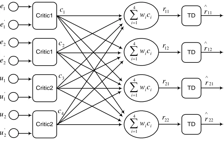
In our paper we present a new block diagram for critic, and we assigned the ETDLC (Emotional Temporal Difference Learning Critics) for it. (See Figure 1 for the schematic of the presented internal ETDLC) [36].
5. AN EMOTION TEMPORAL DIFFERENCE BASED APPROACH TO THE CONTROL OF
DYNAMIC SYSTEMS USING AGENT CONCEPT
In this section we design an intelligent controller based on the concepts considered in the previous
1
e
' 1
e
2
e
' 2
e
1
u
' 1
u
2
u
' 2
u
Critic1
Critic1
Critic2
Critic2
∑
=4
1 i
i i
c
w
∑
=4
1 i
i i
c
w
∑
=4
1 i
i i
c
w
∑
=4
1 i
i i
c
w
1
c
r
11TD 11
∧
r
2
c
3
c
4
c
12
r
TD 12
∧
r
21
r
TD 21
∧
r
22
r
TD 22
∧
r
Figure 1. Schematic of the presented internal ETDLC.
Sensors
Learning Element
Controller
Actuator
To the Palnt (Control Signal)
r internal
NEW
r
Emotional Critics with Temporal Difference Learning
Output Signals from the plant To Other
Agents
From Other Agents
Agents
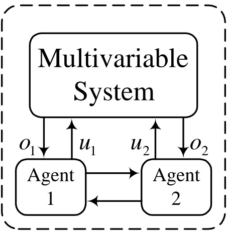
sections. Figure 2 shows the proposed agent’s components and their relation with each other based on the idea presented in [20]. As it can be seen, the agent is composed of five components. It perceives the states of the system through its sensors and also receives some information provided by other agents, then influences the system by providing a control signal through its actuator. The emotional critics with temporal difference learning assess the behavior of the control system (i.e. criticize it) and provide the emotional signals for the controller and that assigned the credit for the prior data for avoiding the curse of dimensionality. According to these emotional signals, the controller produces the control signal with the help of the Learning element, which is adaptive emotional temporal difference learning. Inputs of this learning element are the emotional signals provided by both the agent’s critics and other critics and also some knowledge provided by the controller.
The numbers of the agents assigned here are determined based on the numbers of the inputs of the system. The numbers of the outputs of the system are effective in determining the number/structure of the system’s critics, which their role is to assess the status of the outputs. (See
Figure 3 for the schematic of the presented approach when applied to a 2input – 2output control system).
We now develop the controller structure for the multivariable systems, in general.
In the general case of multivariable systems, each agent consists of a neurofuzzy controller, which has an identical structure to other controllers, i.e. four layers for each one. The first layer’s task is the assignment of inputs’ scaling factors in order to map them to the range of [-1, +1] (the inputs are chosen as the error and the change of the error in the response of the corresponding output). In the Second layer, the fuzzification is performed for each input assigning five labels for each one. For decision-making, max-product law is used in layer 3. Finally, in the last layer, the crisp output is calculated using Takagi- Sugeno formula [21],
)
n
,
,
2
,
1
i
for
(
u
)
c
x
b
x
a
(
u
y
p
1 l
il
il p
1 l
2 i il 1 i il il
i
K
=
+
+
=
∑
∑
= =
(1)
where x and i1 xi2 are inputs to the controller, i, n, uil, p, and yi are the index of the controller, number
of controllers, l’th input of the last layer, number of rules in the third layer and output of the controller, respectively and ail’s, bil’s and cil’sare
parameters to be determined via learning.
For each output, a critic is assigned whose task is to assess the control situation of the output and to provide the appropriate emotional signal. The role of these critics is very crucial here as the eliminating of the unwanted cross-coupled effects of the multivariable control systems is very much dependent on the correct operation of these critics. Here, all the critics have the same structure as of a PD fuzzy controller with 5 labels for each input and 7 labels for the output. Inputs of the critic are error of the output and its derivative and its output is the corresponding emotional signal. Deduction is p e r fo r me d by ma x - pr od u ct l a w a n d fo r defuzzification, the centroid law is used.
Multivariable
System
Agent
1
1
u
u
2
1
o
o
2
Agent
2
To put it in a nutshell, the relationship between agent, neuro-fuzzy, PD fuzzy, MELI controller and critic can be started as follows:
The complex formed by critic and MELIC is called Agent, characteristics of which are desired in detail. However, the basis of implementing MELIC is a neuro-fuzzy system with the previously specified characteristics; the implementation basis of critic, on the other hand, is a PD fuzzy system. The emotional signals provided by these critics contribute collaboratively for updating output layer’s learning parameters of each controller. The aim of the control system is the minimization of the sum of squared emotional signals.
In order to achieve control goals, first, a proper error function should be defined so that it counts for the line conditions in the outputs. Another thing to be taken into consideration is that its sensitivity to the error decreases in the outputs might not be equal. Therefore, it is better to reflect this sensitivity in the output function by assigning different weights in defining these factors, two things should be noted.
First, the factors must be chosen in a way that the convergence algorithm doesn’t pose any problem. Second, a change in each of the factors will change the value of the respective output variable. Formulae 2 to 9 deal with the above mentioned facts.
Accordingly, first we describe the error function
E as follows,
)
r
(
K
E
12 j2j m 1 j
∑
==
(2)where r is the output signal of j’s critic, Kj j is the
corresponding output weights and m is the total number of outputs (for the special case of SISO systems, Kj =1 and m=1)
For the adjustment of controllers’ weights the steepest descent method is used,
)
n
,
,
2
,
1
i
(
E
i ii
∂
ω
=
K
∂
η
−
=
ω
∆
(3)where ηi the learning rate of the corresponding neurofuzzy controller and n is is the total number of controllers.
In order to calculate the RHS of (3), the chain
rule is used,
(
i 1,..., n and j 1,2,..., m)
u u y y r r E E m 1 j i i i j j j j i = = ω ∂ ∂ ⋅ ∂ ∂ ⋅ ∂ ∂ ⋅ ∂ ∂ = ω ∂ ∂∑
= (4)
From (2), we have,
) m , , 2 , 1 j ( r K r E j j j K = ⋅ = ∂ ∂ (5) also, ) m , , 2 , 1 j and n , , 2 , 1 i ( J u y ji i j K K = = = ∂ ∂ (6) where j is the element located at the ji ith column
and jth row of the Jacobian matrix. Assuming: m ,..., 2 , 1 j y y
ej= refj− j = (7)
where e is the error produced in the tracking of j
jth output and yrefj is the reference input (in case number of outputs is greater than the number of inputs, some of yrefj’s are taken as zero as it will be cleared by the inverted pendulum example). Now we have,
j j j j e r y r ∂ ∂ − = ∂ ∂ (8)
Since with the incrimination of error, r will also be incremented and on the other hand, on-line calculation of j j e r ∂ ∂
is accompanied with measurement errors, thus producing unreliable results, only the sign of it (+1) is used in our calculations.
∑
=
∂
ω
∂
η
=
ω
∆
m 1 j i i ji j j i iu
.
J
.
r
.
K
(
i=1,2,K,n andj=1,2,K,m)
(9)Equation 9 is used for updating the learning parameters ail’s, bil’s and cil’s in (1), which is
straightforward.
5. SIMULATION RESULTS
In this section, the proposed method is applied for the control of two dynamical systems. The first one is the controller is applied a to a multivariable linear control plant with strongly coupling (Gas Turbine). Control of a nonlinear chemical reaction is our second example, and control for highly nonlinear and non-minimum phase problem of Inverted Pendulum on a moving cart.
Example 1. ETDL Control of a Gas Turbine
One of the famous examples in multivariable control which has a high coupling is that of the Gas Turbine system. The inputs to the system are the fuel pump excitation in mAmps and nozzle
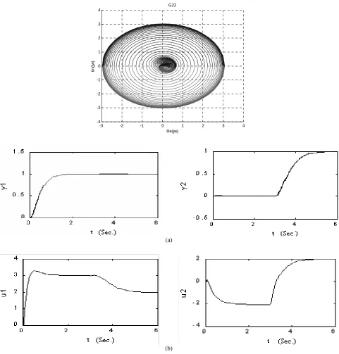
actuator excitation in volts. The outputs of the system are the gas generator speed and the inter-turbine temperature. Applying Laplace transform to the linearized nonlinear differential equation system, the transfer function matrix of the system at 80% gas generator speed and 85% power turbine speed is given as [30].
( ) ( ) ⎥ ⎥ ⎥ ⎦ ⎤ ⎢ ⎢ ⎢ ⎣ ⎡ + + + + + + + + + + + + + + + − + + + = 8 . 18 6 . 111 4 . 116 8 . 20 35 . 9 8 . 25 14 . 7 62 . 1 39 . 9 15 . 9 49 . 0 12 . 2 95 . 1 36 . 2 6 . 13 8 . 12 42 . 1 15 202 . 0 15 . 1 264 . 0 806 . 0 2 3 4 2 2 3 2 2 3 2 s s s s s s s s s s s s s s s s s s s G (10) The block diagram of the control system is
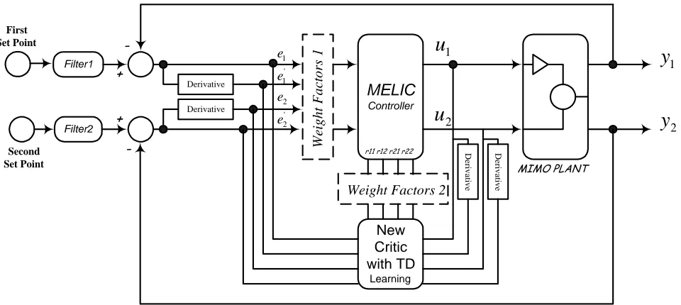
shown in Figure 4.
This system is unstable and has a great deal of coupling. The aim is achieving step response in all of the outputs with a rise time less than 0.3 s in the first output and less than 1.5 s in the second output. Hence, the input filters are selected as follows:
( )
25 . 306 s 35 s 25 . 306 sH1 2
+ +
= (11)
( )
7 s 5 s 7 sH2 2
+ +
= (12)
1
u
Filter1 First Set Point Second Set Point Filter2 MELIC Controller + -MIMO PLANT + - Wei ght Fact ors 1 ' 2 2 ' 1 1 e e e e Derivative DerivativeWeight Factors 2
New Critic with TD Learning Deriv a tiv e Deriv a tiv e
r11 r12 r21 r22
2
u
2 1y
y
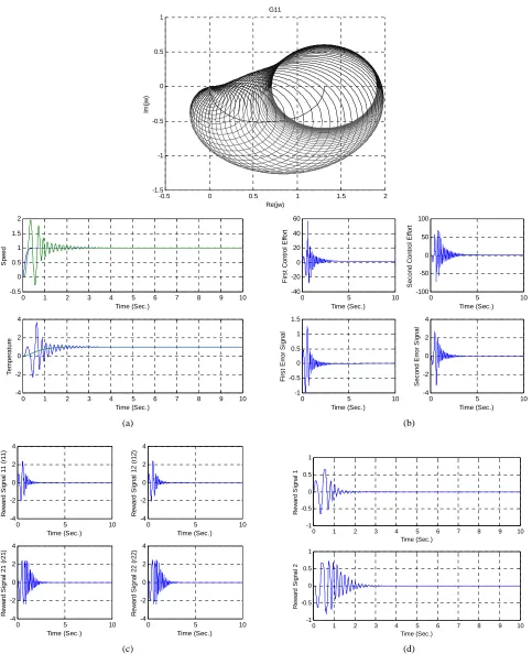
To show gas turbine coupling, Gershgorin bands are manipulated. Gershgorin circles of the transform functions G to 11 G22 are illustrated in Figures 5 to 6 respectively.
The step inputs of the system are applied at the times t = 0 and t = 0, respectively. Results are plotted in Figure 5.
The simulation results of step responses for the system rate of 1 rpm and the temperature of 1 degree Kelvin is illustrated in Figure 5(a) and counts for achieving a proper step response and an excellent attenuation in coupling which is much better than the results presented in references like [30]. Furthermore, control effort signals, emotional signals and error signals are illustrated in Figure 5(b), 5(c) and 5(d) respectively. The Implementing Inverse Nyquist Array suggests that control signal in emotional methods is much less than the one in this classic method.
Example 2. ETDL Control of a Chemical
Process
Our second example is focused on thecontrol of an isothermal continuous-stirred tank reactor (CSTR). It’s a highly interactive nonlinear system with the following reactions [24]:
A B
C B
A
2
3 1
k
k k
⎯→ ⎯
⎯→ ⎯ ⎯→ ⎯
(13)
where the reaction rates are given by:
5 . 0 B 3 3 2 B 2 2 5 . 0 A 1
1 k C ,r k C ,r k C
r = = = (14)
In Equation 14, CA and CB are outlet
concentrations of A and B.
The process can be represented by the following differential equations:
2 2 2 5 . 0 1 1 1 1
1 (u v ) Da v Da v
dt
dv = − − +
(15)
5 . 0 . 2 3 2 2 2 5 . 0 1 1 2 2
2 (u v ) Da v Da v Da v
dt
dv = − + − −
(16) In Equations 15 and 16, u1 and u2 represent the
dimensionless quantities of the feed concentrations of A and B, and v1 and v2 respectively represent the
dimensionless quantities of the outlet concentrations of A and B respectively. Assuming Da1=2, Da2=1
and Da3=2, our goal is to control the outlet
concentrations of A and B by adjusting the feed concentrations of A and B.
It is desired to achieve responses with no overshoots while outputs have rise times no more than 1 and 1.5 seconds, respectively. Hence, the transfer functions of the pre-filters are chosen as follows:
16 s 8 s
16 )
s (
H1 2
+ +
= (17)
7 s 5 s
7 )
s (
H2 2
+ +
= (18)
The step inputs of the system are applied at the times t = 0 and t = 4, respectively. The system inputs are applied to the system at t=0 s and t=3 s to test it in different input times. Results are plotted in Figures 6(a) and 6(b).
According to the simulation results, it can be deduced that with the proposed scheme, nonlinearities are also handled as easily as disturbance rejection and dealing with uncertainties. As observed, the input and output lines coincide perfectly.
Example 3: ETDL Control of an Inverted
Pendulum
The cart with an inverted pendulum,shown in Figure 7, is "bumped" with an impulse force, F. Determine the dynamic equations of motion for the system, and linearize about the pendulum's angle, theta = Pi (in other words, assume that pendulum does not move more than a few degrees away from the vertical, chosen to be at an angle of Pi).
For this example and simulation, let's assume that:
c
m
mass of the cart 0.5 kg m mass of the pendulum 0.5 kg b friction of the cart 0.1sec
m N L length to pendulum center of
mass 0.3 m
I inertia of the pendulum 0.006 2
m
kg
×
F force applied to the cart x cart position coordinate
-0.5 0 0.5 1 1.5 2 -1.5 -1 -0.5 0 0.5 1 G11 Re(jw) Im (j w )
0 1 2 3 4 5 6 7 8 9 10
-0.5 0 0.5 1 1.5 2 S pee d Time (Sec.)
0 1 2 3 4 5 6 7 8 9 10
-4 -2 0 2 4 T e m per at ur e Time (Sec.)
0 5 10
-40 -20 0 20 40 60 F irs t C o n trol E ffo rt Time (Sec.)
0 5 10
-100 -50 0 50 100 S e c ond C ont rol E ffo rt Time (Sec.)
0 5 10
-1 -0.5 0 0.5 1 1.5 F irs t E rror S igna l Time (Sec.)
0 5 10
-4 -2 0 2 4 S e c ond E rror S ignal Time (Sec.)
(a) (b)
0 5 10
-4 -2 0 2 4 R e w a rd S ign al 1 1 (r 1 1 ) Time (Sec.)
0 5 10
-4 -2 0 2 4 R e w a rd S ign al 1 2 (r 1 2 ) Time (Sec.)
0 5 10
-4 -2 0 2 4 R e w a rd S ig nal 21 ( r21 ) Time (Sec.)
0 5 10
-4 -2 0 2 4 R e w a rd S ig nal 22 ( r22 ) Time (Sec.)
0 1 2 3 4 5 6 7 8 9 10
-1 -0.5 0 0.5 1 Re wa rd S ig n a l 1 Time (Sec.)
0 1 2 3 4 5 6 7 8 9 10
-1 -0.5 0 0.5 1 Re wa rd S ig n a l 2 Time (Sec.)
(c) (d)
The problem of balancing an inverted pendulum on a moving cart is a good example of a challenging multivariable situation, due to its highly nonlinear equations, non-minimum phase characteristics and the problem of handling two
outputs with only one control input [25] (the position of cart is sometimes ignored by the researchers [26]). Here, the dynamics of the inverted pendulum are characterized by four variables: θ (angle of the pole with respect to the
-3 -2 -1 0 1 2 3 4
-4 -3 -2 -1 0 1 2 3 4
G22
Re(jw)
Im
(j
w
)
(a)
(b)
vertical axis), θ& (angular velocity of the pole), z (position of the cart on the track), and z& (velocity of the cart). The behavior of these state variables is governed by the following two second-order differential equations [21]:
) m m
Cos * m ( * l
) m m
Sin * * l * m F ( * Cos Sin g
c 2 3
4
c 2 .
+ θ −
+
θ θ −
− θ + θ ∗ =
θ⋅⋅ (20)
m m
) Cos * Sin * ( * l * m F z
c
.. 2
. ..
+
θ θ − θ θ +
= (21)
where g (acceleration due to gravity) is 9.8 2 s m , mc (mass of cart) is 1.0 kg, l(half-length of pole) is
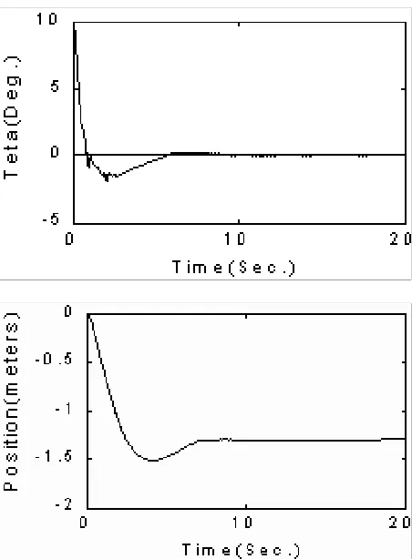
0.5 m, and F is the applied force in Newton. Our control goal is to balance the cart, yet keep the z not further than 2.5 meters from its original position. We use a single agent here, which provides the force F to the system and applies two emotional critics to assess the output. The first one criticizes the situation of the pole and the second one does the same for the cart’s velocity. Both critics are satisfied when inputs to them are zero (i.e. the pendulum is balanced and the cart has no velocity). The results of simulation for initial condition θ0= 10 deg. are presented in Figure 8.
This shows that after nearly six seconds the pole is balanced and the cart is stopped successfully around 1.4 meters from original position.
Which means that when the value of θ=0 and position=1.4 meters the system under control by means of MELIC and Critic based on temporal difference learning, was able to achieve balance 1.4 meters away from its base position whit a lot of effort.
This is because the inverted pendulum has reached 0θ= degree and is completely stable on the cart.
6. CONCLUSIONS
In this paper, the emotional learning based intelligent control scheme was applied to dynamic plants. Also the performance of the proposed algorithm was investigated by several benchmark Figure 8. Responses of variables of example (From left to right: pole’s angle and cart’s position).
θ
F
l
c
m
0
m
x
examples. The main contribution of the proposed generalization is to provide the easy to implement emotional temporal difference learning technique for dealing with dynamic (especially multivariable) control systems where the use of other control methodologies (especially intelligent control methods) is sometimes problematic [27][31].
On the negative side, it should be pointed out that only a very simple learning algorithm has been used throughout this paper. Although this stresses the simplicity and generality of the proposed technique, more complex learning algorithms involving time credit assignments [28] and temporal difference [29][32][35] or similar methods might be called for when processes involve unknown delays.
Considering the achievements of emotional control, this paper seeks to answer more, complex issues and fulfill more objectives. To do this, capability of the learning module of Emotional temporal difference controllers have been dynamically increased for credit assignment by means of temporal difference learning. In addition, multi objective controls, which have been gathered, using the defined emotional signal, pass the critic so that the assigned controller can select the desirable characterization. For showing the practicality of the applied system, we have employed it for developing Gas Turbine control. A gas turbine is a multi variable system with strongly coupling, for which it is difficult to design a good controller, even in a model-oriented form. The results of applying the suggested controller that in addition to the parameters like error and control effort signal being criticized the output has a desired speed and least maximum over shoot in tracking the input.
7. REFERENCES
1. Simon, H. A. and Associates, “Decision Making and Problem Solving”, Interfaces, Vol. 17, (1987).
2. Balkenius, C. and Moren, J., “A Computational Model of Context Processing”, In: Proceedings of the 6th
International Conference on Simulation of Adaptive Behavior, Cambridge, (2000).
3. El-Nasr, M., Loerger, T. and Yen, J., “Peteei: A Pet with Evolving Emotional Intelligence”, Autonomous Agents99, (1999), 9-15.
4. Velasquez, J., “A Computational Framework for Emotion-Based Control”, In: Proceedings of the Grounding Emotions in Adaptive Systems Workshop SAB’98, Zurich, Switzerland, (1998).
5. Fatourechi, M., Lucas, C. and Sedigh, A. K., “An Agent-Based Approach to Multivariable Control”, In the Proceedings of IASTED International Conference on Artificial Intelligence and Applications, Marbella, Spain, (September 4-7, 2001), 376-381.
6. Fatourechi, M., Lucas, C. and Khaki Sedigh, A., “Reducing Control Effort by Means of Emotional Learning”, In: The Proceedings of 9th Iranian Conference on Electrical Engineering (ICEE2001), Tehran, Iran, (2001), 41-1 to 41-8.
7. Fatourechi, M., Lucas, C. and Khaki Sedigh, A., “Reduction of Maximum Overshoot by Means of Emotional Learning”, In: The Proceedings of 6th Annual CSI Computer Conference, 2001, Isfahan, Iran, 460-467 8. Lucas, C. and Jazbi, S. A., “Intelligent Motion Control of
Electric Motors with Evaluative Feedback”, Cigre98, Cigre, France, (1998),1-6. (???: 11-104)
9. Lucas, C., Jazbi, S. A., Fatourechi, M. and Farshad, M., “Cognitive Action Selection with Neurocontrollers”,
Third Iran-Armenia Workshop on Neural Networks, Yerevan, Armenia, (2000).
10. Von Altrock, C. and Gebhardt, J., “Recent Successful Fuzzy Logic Applications in Industrial Automation”, In: Proceedings of the Fifth IEEE International Conference, Vol. 3, (1996), 1845-1851.
11. Lin, C. T. and Lee, C. S. G., “Neural-Network Based Fuzzy Logic Control and Decision System”, IEEE Transactions on Computers, Vol. 40, No. 12, (1991), 1320-1327.
12. Maes, P. (ed.), “Designing Autonomous Agents: Theory and Practice from Biology to Engineering and Back”, The MIT press, London, (1991).
13. Rolls, E. D., “The Brain and Emotion”, Oxford University Press, (1998).
14. Barto, A. G., Sutton, R. S. and Anderson, C. W., “Neurolike Adaptive Elements that can solve Difficult Learning Control Problems”, IEEE Transactions on Systems, Man and Cybernetics, SMC-13, (1983), 834-846.
15. Galloti, K. M., “Cognitive Psychology in and out of Laboratory”, (2nd ed.), Brooks/Cole, Pacific Grove, CA, (1999).
16. Kentridge, R.W. and Aggleton, J. P., “Emotion: Sensory Representations, Reinforcement and the Temporal Lobe”,
Cognition and Emotion, Vol. 4, (1990), 191-208. 17. Berenji, H. R. and Khedkar, P., “Learning and Tuning
Fuzzy Logic Controller Through Reinforcements”, IEEE
Transactions on Neural Networks, Vol. 3, (1992), 724-740
18. Wooldridge, M. and Jennings, N., “Intelligent Agents: Theory and Practice”, The Knowledge Engineering Review, Vol. 10, No. 2, (1995), 115-152.
19. Wooldridge, M., “Intelligent Agents”, in G. Weiss (Ed.),
Multiagent Systems: A modern approach to Distributed Artificial Intelligence, (London: MIT Press, 1999), 27-77
(1995).
21. Takagi, T. and Sugeno, M., “Derivation of Fuzzy Control Rules from human operator’s control actions”, Proc. IFAC Symp.on Fuzzy Information, Knowledge Representation and Decision Analysis, (1983), 55-60. 22. Cheng, C. C. Liao, Y. K. and. Wanq, T. S, “Quantitative
Design of Uncertain Multivariable Control System with an Inner-Feedback Loop”, In: IEE Proceedings on Control Theory Applications, Vol. 144, (1997), 195-201. 23. Fatourechi, M., “Generalization of Emotional Learning
(to Multivariable and Multi-objective Systems)”, M.S Thesis, University of Tehran, (June 2001)
24. Zhao, R. and Govind, R., “Membership Function-Based Fuzzy Model and its Application to Multivariable Nonlinear Model-Predictive Control”, In: Proceedings of the Third IEEE Conference on Computational Intelligence, Vol. 3, (1994), 1586-1591.
25. Cannon, R. H., “Dynamics of Physical Systems”, McGraw-Hill, New York, (1967).
26. Jang, J. S., “Self-Learning Fuzzy Controllers Based on Temporal Back Propagation”, IEEE Transactions on Neural Networks, Vol. 3, No. 5, (1992), 714-723. 27. Lee, P. G., Lee, K. K. and Jeon, G. J., “An Index of
Applicability for the Decomposition Method of Multivariable Fuzzy Systems”, IEEE Transactions on Fuzzy Systems, Vol. 3, (1995), 364-369
28. Sutton, R. S., Barto, A. G., “A Temporal – Difference Model of Classical Conditioning”, In: Proceedings of 9th
Annual Conference on Cognitive Science, New Jersey, (1987), 355-378.
29. Sutton, R. S., “Learning to Predict by the Method of Temporal Differences”, Machine Learning, Vol. 3,
(1988), 9-44.
30. Patel, R. V. and Munro, M., “Multivariable System Theory and Design”, Pergamon press, (1984).
31. Abdi, J., Lucas, C., Sedigh, A. K. and Khalili, A. F., “Truncating Temporal Differences in Control”, 11th
International Conference on Electrical Engineering,
ICEE’03, Shiraz, Iran, (2003).
32. Abdi, J., Lucas, C. and Sedigh, A. K., “Application of Temporal Difference Learning in Control”, M.S Thesis, Uni. of Tehran, (February 2003).
33. Gordon, G. J., “Stable Function Approximation in Dynamic Programming”, In Proceedings of the 12th
International Conference on Machine Learning (ML-95), Morgan Kaufmann, (1995).
34. Sutton, R. S., “Temporal Credit Assignment in Reinforcement Learning”, PhD Thesis, Department of Computer and Information Science, University of Massachusetts, (1984)
35. Sutton, R. S., “Learning to Predict by the Methods of Temporal Differences”, Machine Learning, Vol. 3, (1988), 9-44.
36. Abdi, J., Lucas, C., Sedigh, A. K. and Fatourechi, M., “Multivariable Systems Temporal Difference Emotional Control”, Journal of Faculty of Engineering, Vol.38, No.1, (May 2004), 51-62.
37. Abdi, J., Khalili, A. F., Lucas, C. and Sedigh, A. K., “The Role of Truncated Temporal Difference with Function Approximation in Decreasing the Required Time and Costs of Reinforcement Learning Computations”, IAEEE