JIEM, 2015 – 8(1): 217-232 – Online ISSN: 2013-0953 – Print ISSN: 2013-8423 http://dx.doi.org/10.3926/jiem.1363
Resource Scheduling of Workflow Multi-instance Migration
Based on the Shuffled Leapfrog Algorithm
Yang Mingshun, Gao Xinqin, Cao Yuan, Liu Yong, Li Yan
Faculty of Mechanical and Precision Instrument Engineering, Xi’an University of Technology (China)
[email protected], [email protected], [email protected], [email protected], [email protected]
Received: December 2014 Accepted: February 2015
Abstract:
Purpose:
When the workflow changed, resource scheduling optimization in the process of the
current running instance migration has become a hot issue in current workflow flexible
research; purpose of the article is to investigate the resource scheduling problem of workflow
multi-instance migration.
Design/methodology/approach:
The time and cost relationships between activities and
resources in workflow instance migration process are analyzed and a resource scheduling
optimization model in the process of workflow instance migration is set up; Research is
performed on resource scheduling optimization in workflow multi-instance migration, leapfrog
algorithm is adopted to obtain the optimal resource scheduling scheme. An example is given to
verify the validity of the model and the algorithm.
Findings:
Under the constraints of resource cost and quantity, an optimal resource scheduling
scheme for workflow migration is found, ensuring a minimal running time and optimal cost.
Originality/value:
A mathematical model for resource scheduling of workflow multi-instance
migration is built and the shuffled leapfrog algorithm is designed to solve the model.
1. Introduction
The sustainable development of business enterprise is threatened by the contention between rapidly-increasing business volume and limited enterprise resources. As the core technology of process modeling and management, workflow technology is of key importance for improving information level, production and operations management, operation efficiency, response ability to the external environment change and market competitiveness of manufacturing enterprises (Xu, 2014). Workflow resource scheduling is the primary concern of workflow management systems. To determine how resources can be most appropriately used to execute workflow instances, thereby improving the execution efficiency of business processes has been the primary focus.
Due to increasing market competitiveness and the complex and ever-changing demands of enterprise, uncertainty and variability have become significant features of business enterprise (Feifan & Xuanxi, 2006). Workflow instance migration can effectively solve the problem of workflow dynamic change. As the workflow changes, the running instance will choose an appropriate migration strategy (direct migration, rollback migration, or no migration) according to the very status (Gao, Xu, Wang, Li, Yang & Liu, 2013). During the process of workflow migration, the workflow process model will change; the resources relevant to the original process model will also change, such as resource rebuilding or canceling, which makes the resource scheduling optimization in the workflow migration process very important. How to migrate currently running instances and schedule resources during instance migration process has become widely debated issue in workflow flexibility research.
Aiming to resolve the grid workflow scheduling problem, Sucha Smanchat et al. proposed a scheduling algorithm for a multi-parameter sweep workflow instance based on resource competition (Smanchat, Indrawan & Ling, 2011). Rizos Sakellariou et al. considered resource allocation problems to be a single activity instance of the workflow and set the earliest completion time for a certain activity instance as the goal of their resource scheduling method (Sakellariou, Zbao, Tsiakkouri & Dikaiako, 2007). R. Buyya analyzed the relationship between the overall deadline of a workflow instance and the load of an activity instance in order to estimate the deadline for each activity’s running time. The workflow instance resource scheduling problem has been developed into multiple scheduling problems (Yu, Buyya & Tham, 2005). G. B. Tramontina et al. adopted a variety of allocation rules (First In First Out, Earliest Due Time, Service In Random Order, and Shortest Processing Time) in order to schedule resources among multiple workflow instances (Tramontina & Wainer, 2005).
considered. Zhang Lijun solved the problem of dynamic task allocation using sub-processes; although the design and execution of the sub-processes were given in this method, it paid less attention to resource task scheduling (Lijun, Jun & Tao, 2009). Liu Subo established a resource-task allocation model, and designed a process-scheduling decision system based on workflow management, resolving the problems arising from resource optimization scheduling and exception handling (Subo, Jianchong & Haizhu, 2011). Deng Tieqing et al. studied the personal worklist scheduling problem in an environment of dynamic execution of workflow instances, and proposed a personal worklist resource scheduling algorithm based on a genetic algorithm; this method studied resource scheduling of multiple activity instances in a single process, but not in resources scheduling of multiple process instances (Deng, Ren & Liu, 2012). Yang Mingshun et al. established a workflow multi-instance resource optimization model based on queuing theory and used the simulated annealing intelligent algorithm to solve the model (Yang, Han, Gao & Liu, 2012). This model solved the resource optimization problem with the constraints of resource cost and state as the instances were running, but the resolution lacked the consideration of resource competition and its advantages and disadvantages.
2. Resource Scheduling Modeling in Instance Migration Process
2.1. Workflow Instance Migration Process Analysis
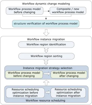
The workflow instance migration process primarily includes modeling of dynamic change of workflow, workflow instance migration, and resource scheduling optimization.
(1) Modeling of dynamic change of workflow refers to build a new or composite workflow process model of the changed workflow process based on the original workflow model. Firstly, it is required to analyze the change style of the workflow, then the new/composite workflow process models corresponding to the original ones are built, finally the structures of the newly built models are verified to determine whether any conflict or error exists. Only no conflict or error existing in the workflow structure, the new model is reasonable, and the instances run in the original model can migrate.
(3) It is well-known that the successful running of the workflow instances cannot do with appropriate resources, especially in the process of workflow instances migration. Only with the supports of appropriate resources, can the instances migrating be successfully realized. The purpose of workflow resource scheduling is to allocate the right activities to the right activities in right time with right sequence to ensure the every activity of the workflow instances can be executed by the appropriate resource in right time, thus the whole business process can be finished successfully. The resource scheduling results will directly affect the work efficiency, flexibility and service quality of the workflow management system.
The framework of the workflow instance migration process is shown in Figure 1.
Figure 1. Process framework of the workflow instance migration
In the workflow instance migration process, due to uncertain factors such as resource changes and resource release, the dynamic resource scheduling optimization should be applied to the migration instance so that the workflow system can achieve global optimization of resource utilization. By analyzing the relationship between the activities and resources in the workflow instance migration process, certain factors, including the shortest overall activity execution time, the minimum overall activity lag time, the minimum number of activities lagged and the minimum costs that the resource consumed were used as the optimization goals to establish the mathematical model of workflow resource scheduling optimization.
2.2. Resource Scheduling Parameters
(1) Activity i’s lag time (Δti) represents the time difference between the expected activity
completion time and the actual completion time.
(1)
where tei is the expected completion time of activity i and tfi is the actual completion time of
the activity. The expected completion time of activity i is the time expected to meet the time requirements or obtain certain time performance. The expected completion time could be set by users or generated by the system.
(2) Activity i’s actual completion time (tfi) represents activity i's actual starting time plus its
execution time.
(2)
where tsi is the starting time, tij is the time resource j spends executing activity i.
(3) The execution time (tij) of resource j, or the time resource j spends executing activity i,
represents the ratio of the workload of activity i to the executive ability of resource j.
(3)
where Wi is the workload of activity i, Aij is resource j’s ability to execute the activity, and
is acorrection coefficient.
(4) The consumption cost (Cij) of resource j in the execution of activity i represents the
(4)
where cj is the average consumption cost of resource j per unit of time, and tij is the time that
resource j spends executing the activity.
(5) The available time of resource j (trj) includes the current time, the idle time of resource i,
and the execution time already allocated to resource j.
(5)
where tvj is the idle time of resource j, tc is the current time, is the overall execution
time already allocated to resource j, and
l
is the number of tasks already been allocated to resource j.(6) In case one resource serves several activities, virtual resources need to be introduced in order to obtain an optimal resolution of the activity and the resource sorting problem. Assuming that resource j needs to participate in β executing activities, β-1 virtual resources of resource j need to be added. The physical and virtual resources are expressed as j.k (k = 0, …,
s - 1). Then, equation (5) could be modified as the following:
(6)
Where tpjq is the allocated time that resource j spends executing activity q.
(7) The actual starting time of the activity depends on the available time of the resource.
(7)
Where trj.k is the available time of resource j.k, and j.k is the resource that executes activity i.
Free time of a resource refers to a moment after which the resource j will not participant in execution of any activity and can be represented with tvj. Available time of a resource refers to
the moment that the resource j can participant in the execution of a new activity and can be represented with tvj.
When an activity needs multi resources to be executed, which means a teamwork. Multi resource execution styles are required to be taken into account. There are mainly four styles: different time and place, same time and place, same time and different place, different time and same place. In the process of workflow instance running, only the time factor of resource executing is considered, thus in the paper the style of same time and place of the resource teamwork is mainly considered.
(8) The execution time ( ) of activity i by team wt depends on the completion time of the
resource that spends the longest time executing the activity.
(8)
where
(wt)h is the modified coefficient of the demanding time that resource member h of teamwt spends executing activity i, is the workload executed by resource (wt)h, and is
the ability of resource (wt)h to complete activity i.
(9) The available time ( ) of team wt depends on the available time of the last available
resource in the team.
(9)
Where |wt| refers to the number of resource contained in wt, (wt)h refers to resource h that
is involved in team wt of activity i.
(10) The matrix elements of lag matrix a, with dimensions m
1, are the set of the presently demanded resource scheduling activities; the values of these elements are expressed as the following:For any activity, when the lag time
ti < 0, yielding a value of element ai = 1 in the lag matrix,the implementation of the activity lags. Otherwise, when ai = 0, activity i is executed normally.
(11) The cost Ci(wt) needed for team wt’s execution of activity i depends on the execution time
of each resource member.
(11)
Where is the modified coefficient of the demanded time for the execution of activity i by resource member h of team wt, is the workload executed by resource member h,
is the ability of resource member h to complete activity i, and is the running cost per unit of the execution of activity i by the resource member.
2.3. Modeling
In a workflow management system, the workflow instance wfk(k=1,...,p) is running, p is the
total number of currently running workflow instances. At a certain moment, the active node
i(i=1,...,m) is to be performed and m is the total number of activities to be performed, the resource j(j=1,...,n) is available that can be allocated and n is the total number of resources available. R represents a resource set, Ri R represents the resource set that could be
allocated to task i, and cjrepresents the execution cost of resource j per unit of time.
In order to select the appropriate resource ri(ri=1,...,n) for the execution of activity i, thereby
ensuring the shortest total activity execution time, the shortest total activity lag time, the fewest lag activities, and the lowest total resource consumption cost, the following formulas were derived:
The shortest total activity execution time is
(12)
The shortest total activity lag time is
The fewest lag activities is
(14)
The lowest total resource consumption cost is
(15)
s.t.
(16)
(17)
(18)
(19)
(20)
(22)
(23)
(24)
where wi is the importance of the current activity in the running instance wfk.
3. Leapfrog Algorithm
Shufflered leapfrog algorithm (SFLA) belongs to a class of heuristic swarm intelligence optimization algorithms which triggers a heuristic search for an optimal solution using a certain mathematical function (Peng-jun & San-yang, 2009). The algorithm combines the advantages of both Memetic algorithm and particle swarm optimization algorithm; some of the advantages include relatively simple concept, relatively few parameters, strong global optimization capability, high computing speed and robustness (Zhu & Zhang, 2014). Leapfrog algorithm has been successfully applied to some technology fields, such as multi-objective optimization technology, traffic control, cluster analysis, and some combinatorial optimization problems.
In the leapfrog algorithm, the population is composed of many “frogs” with the same structure, each representing a particular solution. The total population is divided into many sub populations called memeplexes. Different sub-populations (memeplexes) can be thought of as collections of “frogs” with different cultures; as such, these memplexes are executed in accordance with certain local search strategies. In each sub-population (memeplex), each “frog” has its own ideas, but is also affected by the others in its community. After a certain memeplex evolution and jumping process, the cultural ideas of the various sub-populations become mixed during computation; the local search and jumping are executed until the convergence criteria are met.
Step 1: Initializing parameters. Selecting the appropriate number m of memeplex and frog number n of every memeplex, then the number of the population is F = m
n.Step 2: Initializing population. F frogs X(1), X(2),...,X(F) are generated randomly in the feasible region
, let d be a dimension variable, the frog i can be represented as X(i) =
Xi1,Xi2,...,Xid
x(i) and the fitness function is f(i) = F(X(i)).Step 3: Sequencing frogs. The F frogs are ordered according the fitness values and storage with, the best frog Xg = U(1) is recorded.
Step 4: Grouping the frogs and storing in different memeplex. Dividing U into m memeplex,
Y1, Y2,…, Ym, there are n frogs in every memeplex. The frogs are allocated according to the
formula
Step 5: Evolving of memeplex. In a memeplex, every forg will be affected by the others and will evolve through the memeplex, the frog will leap toward the targeting positon.
Step 6: Leaping and moving. The frogs will leap and move among the memeplex, after certain Memeplex evolutions are executed in every memeplex, the frog groups Y1, Y2,…, Ym are merged
into U and reordering is carried out, the best frog Pg of the whole population is updated.
Step 7: Judging the algorithm termination condition. If the iteration meets the termination condition, the iteration end and the best frog is output, otherwise executing step 4 again.
4. Illustrative Example
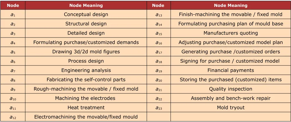
Figure 2 is a workflow process model of the mold processing of a domestic mold manufacturing enterprise; the definition of each active node is shown in Table 1.
Figure 2. Business process model for mold project management
Node Node Meaning Node Node Meaning
a1 Conceptual design a13 Finish-machining the movable / fixed mold
a2 Structural design a14 Formulating purchasing plan of mould base
a3 Detailed design a15 Manufacturers quoting
a4 Formulating purchase/customized demands a16 Adjusting purchase/customized model plan
a5 Drawing 3d/2d mold figures a17 Generating purchase /customized orders
a6 Process design a18 Signing for purchase / customized model
a7 Engineering analysis a19 Financial payments
a8 Fabricating the self-control parts a20 Storing the purchased (customized) items
a9 Rough-machining the movable / fixed mold a21 Quality inspection
a10 Machining the electrodes a22 Assembly and bench-work repair
a11 Heat treatment a23 Mold tryout
a12 Electromachining the movable/fixed mould
Table 1. Active node definitions
Figure 3. Compound workflow process model
Notes deletion: moving and fixed mold electrical processing (a12), Node structure parallelization: purchase
Suppose a set of migration nodes of the multiple instances is Ai = {a1, a2, a3, a4, a5, a6, a7, a8,
a9, a14, a15, a16}. Table 2 shows the relationships between the allocated active nodes and the
time-related resources available for the current scheduling time. In order to facilitate expression and calculation, each of the time parameters in the Table 2 was converted to a relative time scale, and the current scheduling time was set to 0.
The expected time tei of activity i was used to denote the expected completion time of each
activity, and the time resource j spent executing activity i was obtained in accordance with the preference of the resources, the resource capacity and workload of the activity.
Activity i a1 a2 a3 a4 a5 a6 a7 a8 a9 a14 a15 a16 a17
Expected moment tei
Resource j 5 7 9 15 13 21 14 29 26 15 8 5 14
r1 4 5 8 - - -
-r2 3 9 11 - - -
-r3 7 12 15 - - -
-r4 6 8 12 - - -
-r5 10 4 10 - - -
-r6 - - - - 15 22 - - -
-r7 - - - - 12 24 - - -
-r8 - - - - 13 - - -
-r9 - - - 18 - - -
-r10 - - - 18 - - -
-r11 - - - 10 - - - 13
r12 - - - 14 - 5
-r13 - - - 13 - 5
-r14 - - - 10 -
-r18 - - - 24 25 - - -
-r19 - - - 30 26 - - -
-r20 - - - 42 26 - - -
-r21 - - - 22 - - - -
-Table 2. Time information for resource-activities
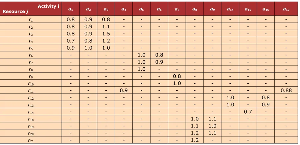
Activity i
Resource j a1 a2 a3 a4 a5 a6 a7 a8 a9 a14 a15 a16 a17
r1 0.8 0.9 0.8 - - -
-r2 0.8 0.9 1.1 - - -
-r3 0.8 0.9 1.5 - - -
-r4 0.7 0.8 1.2 - - -
-r5 0.9 1.0 1.0 - - -
-r6 - - - - 1.0 0.8 - - -
-r7 - - - - 1.0 0.9 - - -
-r8 - - - - 1.0 - - -
-r9 - - - 0.8 - - -
-r10 - - - 1.0 - - -
-r11 - - - 0.9 - - - 0.88
r12 - - - 1.0 - 0.8
-r13 - - - 1.0 - 0.9
-r14 - - - 0.7 -
-r18 - - - 1.0 1.1 - - -
-r19 - - - 1.1 1.0 - - -
-r20 - - - 1.2 1.1 - - -
-r21 - - - 1.2 - - - -
The cost that resource j spent executing activity i per unit of time is shown in Table 3. The cost of resource execution per unit of time was determined by the properties of the resource itself.
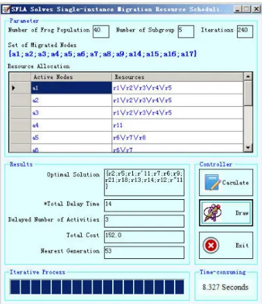
In order to develop the optimization mathematical model for scheduling described in section 2.3, the optimal resource scheduling results were solved using the designed leapfrog algorithm. First, the parameters were initialized; the number of frog populations was set to 40, the ethnic memeplex number was set to 5, the number of frogs in each memeplex was set to 8, and the maximum number of iterations was set to 250. Next, the C# programming language was used to write the algorithm program. The process used to solve the scheduling problem is shown in Figure 4, and the fitness value curve of the possible solutions for each generation is shown in Figure 5.
Figure 4. Resource scheduling optimization module for multi-instance migration
The scheduling result (S ) is equal to {r2,r5,r1,r (1)11,r7,r6,r9,r21,r18,r13,r14,r12,r (2)11}, the total
activity lag time is equal to f2({ S3}) = 14, the number of lag activities is equal to f3({S3}) = 3, and the consumption cost is equal to f4({S3}) = 152.0, where r (1)
1 1 and r (2)11
represent the execution of active nodes a4 and a17 by resource r11, and the order of execution is
a4, a17.
5. Conclusion
In this paper, the resource scheduling optimization of workflow instance migration was analyzed. In order to investigate the resource scheduling problem of workflow multi-instance migration, time and cost relationships of activities and resources were analyzed. Certain factors, including the shortest overall activity execution time, minimum overall activity lag time, minimum number of lag activities, and minimum resource consumption cost were used to establish a workflow resource scheduling optimization mathematical model for workflow instance migration. A leapfrog algorithm was implemented to solve the optimal resource scheduling problem. Specific examples were listed to validate the proposed mathematical resource scheduling model and designed algorithm. The results showed that, under the constraints of resource cost and quantity, an optimal resource scheduling scheme for workflow migration can be found, ensuring a minimal running time and optimal cost. On the other hand, only the same-time working style of multi resources executing workflow activity is considered, case of activity executed with other working style should be further studied. Also, only resource scheduling of multi instance migration in a single workflow model is considered, resource scheduling optimization of multi instance migration in multi workflow models should be further studied.
Acknowledgments
This research is supported by Nature Science Foundation of China (Grant No. 61402361), Technology Project of Shaanxi province, China (Grant No. 14JK1521), Science and Technology Research of Shaanxi province, China (Grant No. 2012KJXX-34), Science and Technology Innovation Team for Youth of Xi’an University of Technology, China (Grant No. 102-211408) and Scientific Research Plan of Xi’an University of Technology, China (Grant No. 102-211305).
References
Deng, T.Q., Ren, G.Q, & Liu, Y.B. (2012). Genetic Algorithm Based Approach to Personal Worklist Resource Scheduling. Journal of Software, 23, 1702-1716.
Feifan, K., & Xuanxi, N. (2006). Wokflow Modeling Design Based on Petri Net and UML. Journal of Nanjing University of Aeronautics & Astronautics, 38, 121-125.
Gao, X., Xu, L., Wang, X., Li, Y., Yang, M., & Liu, Y. (2013). Workflow process modelling and resource allocation based on polychromatic sets theory. Enterprise Information System, 7, 198–226. http://dx.doi.org/10.1080/17517575.2012.745617
Lijun, Z., Jun, M., & Tao, Y. (2009). Research and implementation of dynamic task scheduling based on workflow. Computer Engineering and Design, 30, 2533-2540.
Peng-jun, Z, & San-yang, L. (2009). Shuffled frog leaping algorithm for solving complex functions. Application Research of Computers, 26, 2435-2437.
Sakellariou, R., Zbao, H., Tsiakkouri, E., & Dikaiako, M. (2007). Scheduling workflows with budget constraints. Integrated Research in Grid Computing, 5, 189-202.
http://dx.doi.org/10.1007/978-0-387-47658-2_14
Shengwen, L., & Junfang, G. (2010). Research on Workflow Schedule Model based on Fuzzy Theory. Application Research of Computers, 27, 131-133.
Smanchat, S., Indrawan, M., & Ling, S. (2011). A Scheduler based on Resource Competition for Parameter Sweep Workflow. Procedia Computer Science, 4, 176-185.
http://dx.doi.org/10.1016/j.procs.2011.04.019
Subo, L., Jianchong, Z., & Haizhu, X. (2011). Resource Scheduling based on Workflow Model.
Fire Control & Command Control, 36, 126-130.
Tramontina, G.B, & Wainer, J. (2005). Modeling the Behavior of Dispatching Rules in Workflow Systems: A Statistical Approach. Computer Science, 8, 208-215.
Xu, L.D. (2014). Advances in e-business engineering management. Information Technology and Management, 15, 65-67.
Yang, M., Han, Z., Gao, X., & Liu, Y. (2012). Resource Allocation Optimization of Workflow with Multi-instance and Multi-resource Based on Queuing Theory. International Review on Computers and Software, 7, 2384-2393.
Yu, J., Buyya, R., & Tham, C.K. (2005). Cost-based Scheduling of Scientific Workflow Applications on Utility Grids. e-Science and Grid Computing, 4, 147-154.
Zhu, G.Y., & Zhang, W.B. (2014). An improved Shuffled Frog-leaping Algorithm to optimize component pick-and-place sequencing optimization problem. Expert Systems with Applications, 41, 6818-6829. http://dx.doi.org/10.1016/j.eswa.2014.04.038
Journal of Industrial Engineering and Management, 2015 (www.jiem.org)