Irrigation Scheduling with Soil Instruments: Error Levels and Microprocessing Design Criteria

(1)

IRRIGATION SCHEDULING WITH SOIL INSTRUMENTS: ERROR LEVELS AND MIGROPROCESSING DESIGN CRITERIA

J. W. Cary 1/

Two criteria for deciding when a crop should be irrigated are: (1) the depletion of water in the root zone to some predetermined amount, or (2) the

decrease of water potential

at some given depth to a

predetermined level. The

value one chooses for either of these criteria to indicate that irrigation is needed will

depend on soil properties, crop

rooting

characteristics and stage

of plant growth. Functional relations between these

two criteria and produc-tion are

not yet known quantitatively,

thus one cannot say that either ap-proach is inherently better than the other. The effective application of either requires experience and judgment.

Recent years have seen significant

progress in

scheduling irrigation using

meteorological data to calculate the depletion of water in the root zone. The daily potential evaporation from a

full cover reference crop can be calculated

within

a few

percent using

measurements of air temperature, humidity, solar radiation and wind run. • Given an appropriate crop

coefficient curve,

the

evapotranspiration can also be

estimate and the soil water depletion known with varying degrees of accuracy. As an alternative, the

rate of soil water

depletion may

be

directly

measured with

a neutron meter or by gravimetric soil sampling. Gear at al. (1977) used a neutron meter to measure soil water on successive dates and projected soil water depletion with

a

straight line to

a

level where replenishment would be needed. This

gave estimates of the number

of days until irrigation.

Tensiometers, resistance blocks, thermoconductivity sensors, psychrometers and related

instruments

have been occasionally used or proposed for use in auto-matically starting irrigation at some given water potential.

Tensiometers and

gypsum resistance blocks have been available for many years

to help decide when the soil should be

irrigated. Fischback (1978)

reported results of scheduling the irrigation of corn by several different methods

including

resistance blocks and

a

meteorological approach. He

tended to favor the

blocks.

At the present time, a farm manager may schedule irrigation

with soil

water potential instruments. Based on experience, he will extrapolate the soil water change expected in the next few

days, and

arrive at a projected date for irrigation. The recent

evolution of

microprocessors suggests that

a

system might be designed that would automatically read soil water potential instru-ments and predict the day to irrigate using an

appropriate

algorithm. This

could lead to a

level of sophistication for predicting irrigation frequencies comparable to that developing for computer

scheduling with microclimate

data (Wright and Jensen, 1978).

The general patterns of change in

soil water potential with

time at a given depth are shown in Fig. 1.

1/ Soil Scientist,

Agriculture Research Service, U. S. Department of

Agricul-ture, Snake River Conservation Research Center, Kimberly, Idaho 83341.

(2)

TIME

C

1

=

0_

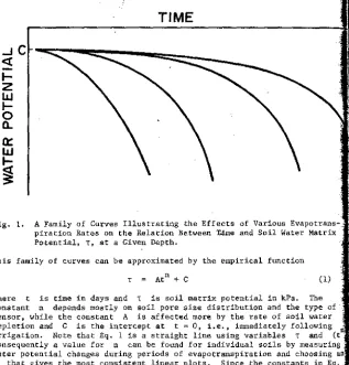
Fig. 1. A Family of Curves Illustrating the Effects of Various

Evapotrans-piration Rates on the Relation Between time and Soil

Water Matrix Potential, T, at a Given Depth.

This family of curves can

be approximated by the empirical function T

=

At n + C

where

t is time in days and

T

is soil matrix potential in kPa. The constant n depends mostly on soil pore size distribution and the type of sensor, while the

constant A is affected more by the rate

of soil water depletion and

C is the

intercept at t 0, i.e., immediately following n

irrigation. Note that Eq. 1 is a straight line using variables

T

and (t

Consequently a value for n can be found for individual soils by measuring water

potential changes during periods of evapotranspiration and choosing an

n that gives the most consistent

linear plots. Since the constants

in Eq. can be calculated from

appropriate data, a microprocessor could be programme

to project irrigation by extrapolating time to some

predetermined

water pote

tial.

The feasibility of such an

undertaking requires an analysis of the inherent

errors with

respect

to the errors

encountered in scheduling with microclimate data and with respect to the level of error that is practical f the grower. Specifically, it comes

down to questions on the applicability o

Eq. 1, the accuracy and reliability of

soil

water potential sensors, and the

spatial variability of soil water in the field.

EXPERIMENTAL PROCEDURES

Data were collected

during two growing seasons on four plots of Portneuf sil

loam soil described in detail by Cary and Rasmussen (1979). Each plot was 2

meters

long and 9 meters wide. Corn,

beans,

sugarbeets

and grass were

grown

the

first year; beans and sugarbeets followed the

second year. The plots

we

irrigated

with corrugates

(except the grass which was border

flooded). Each

plot was sampled

and instrumented on

both ends such

that data collection sit were about 170 meters apart.

There were 8 data collection sites the first season. Each had two permanent

tensiometers at the 30-cm

depth. There were commercial units with 45-cm lon

plastic cylinders connecting the ceramic cups to vacuum gauges. Three gypsum

(3)

resistance blocks2/ were also installed in the rows at the 30-cm depth within a 2-m radius. The resistance of each block was measured five days a week with a 1K Hertz electrical conductivity bridge. Soil

temperatures around each set

of blocks were also measured. Gravimetric soil water measurements at depths of 15, 30, and 45 cm were made from two cores taken about 2 m apart twice weekly at random locations in the rows near the blocks and tensiometers. In the second season, the blocks

were placed at both 15- and 30-cm depths and

their

resistances were

measured twice a week. Three portable rapid response

tensiometers3/ were also inserted twice weekly to measure water

potential

at

the 30-cm depth. These tensiometers were placed at random

not farther

than

2 m apart in

crop rows near the blocks.

-Care was taken to

irrigate

the plots

as uniformly as possible.

Fertility and

cultural practices were in accord

with local

recommendations and

practices.

At the end of the growing season, 4 sites, 2 at each end of the field, were

sampled, taking four undisturbed cores from

each site. Slices

were

taken from

these cores at the

26- to 34-cm depths and

individual

moisture desorption curves measured for each core.

These data were used to calculate pore size

distribution indexes by the method of Cary and Hayden (1974).

RESULTS

The gravimetric soil water measurements

were used to assess

the spatial

vari-ability within the plots

and to compare the variability shown

by the tensi-ometers and blocks. Methods of characterizing soil spatial variability are

not

yet

very well developed,

though this is being addressed by a number of soil scientists

(Rao

et al., 1979 and 'Western Regional Research Committee

155). In this case, the standard deviation was calculated for two or more

observations that should

have been identical. This value was divided by the

mean of the observations to get the coefficient of variation. The average of all the coefficients of variation was then used to characterize the vari-ability (Table 1). This approach reduces the dependence of standard deviation

on the range of the data

observations

since the standard

deviation of water

potential increases rapidly as

the

potential becomes more negative.

The standard deviation of

the water content increases as

the

water content increases, but as pointed out by Ben-Asher (1979),

standard deviation in

general for uniform soils is about 10%

of the water content. Nielson et al.

(1973) found average standard deviation of volumetric water

and 7% in a field study, indicating

a coefficient of variation range

of 13 to 20%. Cassel and Nelsen (1979) also reported the coefficients of variation of

volumetric water contents ranged from 8 to 25% in an intensive field study.

Entries 1, 3, 7 and 9 in Table 1 are measures

of

the short distance

spatial

variability of soil in the test strips. Average values of water potential from each of these local observation sites were averaged and their means used

to characterize the overall spatial

variability of the study

area, i.e.,

entries 2, 4, 5, 8 and 10.

Averaging

several localized

measurements

to get means for

characterizing the overall spatial variability reduces

the error caused by the inherent

variability of the measuring instrument as

demonstrated

2/ Beckman

Instrument Company, Cedar

Grove, New

Jersey.

3/ Soil moisture probe Model 2900, Soil Moisture Equipment Corporation, Santa Barbara, California.

Trade names

and company names are

included for the benefit of the reader

and do not

imply any endorsement or preferential

treatment of the product by the

U. S. Department of Agriculture.

(4)

4.7%

1144

5.4%

582 10.5%

16 5.9%

• 4

20.6%

186 /2.5%

136 25.7%

306 16.6%

102 11.9%

384

9 to 30% by wt.

10 to 28% by wt.

2.4 to 3.6

3.0 to 3.4

- 20 to - 72 kPa

-30 to -150 kFa

- 20 to -900 kPa

- 30 to -800 kPa

- 5 to - 76 kPa

13.3%

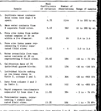
106 - 1 to - 70 kPa Table 1. Coefficients of Variation Associated with Measured Values of Soil

Water Potential,

Water Contents on a Weight

Basis,

and

Soil Pore

Size Distribution Indexes.

...

Mean

Coefficients

Number of

Sample of variation observations Range

of samples

1. Duplicate

water contents

from cores less than 2 m

apart.

2. Mean water contents from

8 separate field sites.

3. Pore size index from

undis-turbed samples at 30 cm

within

a

2-m diameter.

4. Pore size index means

rep-resenting 4 widely

sepa-rated field sites.

5. Water potentials from mean

water contents at 30 cm

representing 8 field sites.

6. Calibration data of 28

individual gypsum blocks.

7. Individual blocks making

up the means shown in

Table 2, columns 2 and 3.

8. Data from columns 2 and 3

in Table 2.

9. Rapid response tensiometers

separated by leas than 2 m.

10. Tensiometer means,

repre-senting 4 widely

sepa-rated field sites.

.--.=

..

.

...

by the reduction in the coefficient from entries 7 to 8. The coefficient in

entry 7 came from 12 blocks, 3 each at 4

widely separated sites in the study area. The coefficient in entry 8 was based on the means of 3 localized bloc

at

each of the 4 separated sites.

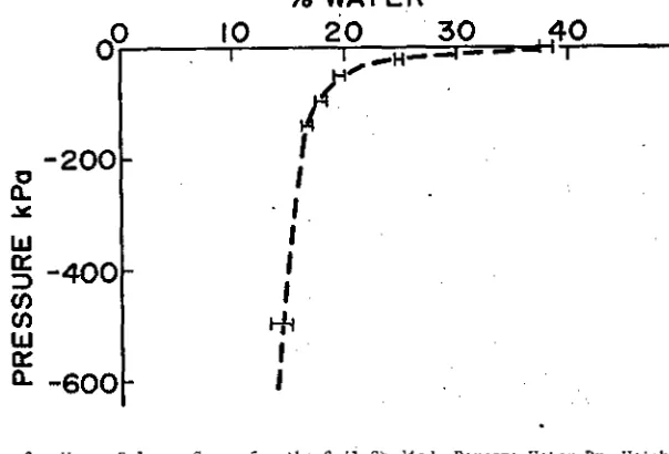
Water potential was estimated.

from the gravimetric water content at the

30-depth, assuming a single water desorption function, Fig. 2, for all four plo

(entry 5, Table 1). The coefficient of variation of these potentials

was 20.6% which was greater

than the coefficient of

variations of

the poten

tials measured with

blocks

or tensiometers (entries 8 and 10). Consequen tly

it appears the inherent

inaccuracies

in measuring soil metric potential

with

gypsum resistance

blocks or tensiometers may be no greater than the inhe rent

spatial

variability in the field.

Particularly

with blocks, the average

resistance

of

several placed near one

another may be used to reduce

the

effect

of their inherent variability.

(5)

% WATER

1

0

20

30

40 1-14

-200

a.

-400

ix

a-

-600

Fig. 2. Water Release Curve for the Soil Studied, Percent Water Dry Weight Basis as a Function of

Pressure in

the Desorption

Chamber. Brackets

Show the Spread of Mean Water Contents from the Four. Sampling Sites. The Pore Size Distribution Indexes Associated With These Data are Given in Table 1.

DISCUSSION

Several problems associated with automating the tensiometers and blocks with

a microprocessor to read out projected irrigation dates were noted during the

experiment and analysis of data. The permanent plastic tube tensiometers were

unsatisfactory for automation because they required weekly service and were sluggish when the soil was drier than -60 kPa. They had to be placed 30 cm

deep• to remain operative for at least the first two-thirds

of some irrigation

cycles. The rapid response tensiometers were better, but even they had to be

recharged once or twice during the

season.

Their effective range was only

down to a bit less than -70 kfa (elevation 1,130 m). Their mobility and rapid

response time were

advantages

insofar as characterizing conditions

in the

field, but considerable

care was required to install them, particularly when the soil surface was dry and slaked into the access holes.

The gypsum resistance blocks also have several inherent problems. They are

temperature dependent. The empirical

equation

R22 == ((T0.011 -1) (T-22) -1- 1] R

(2)

was found from measurements made in a controlled temperature room. It

was

used to correct the observed resistance to the 22°C calibration temperature. A second empirical equation was then developed for the soil water potential

T q.0217 R

22

+ 69.84 In R

22

-3.245

AT---

₂₂ -310.5 (3) where R

is

the measured resistance in ohms, T is

the temperature of the

block °C and R 22 is resistance corrected to 22°C.

(6)

Gypsum blocks also have some wetting and drying hysteresis that may be signif

icant under transient soil water conditions.

Problems were noted at the 30-cm

depth

when irrigation did not quite

increase the

potential to -30 kPa before

rapidly falling again due to soil water extraction. In essence, the blocks

did not always rewet to the level

indicated by gravimetric samples. This problem was less at the

15-cm depth because the soil water content rises

higher following rain

and light

irrigations allowing a more complete block

response. As a consequence, blocks at the 15-cm depth passed through a wider

range of water potentials during each drying cycle than blocks at the 30-cm

depth or tensiometers

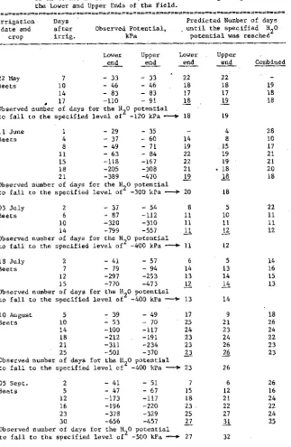
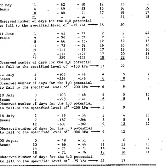
at any depth. This is an advantage for automation and data reduction with a microprocessor.

The mean water potentials from the three temperature corrected blocks at the

15-cm depth are shown in Table 2 for the upper and

lower ends of

the beet and bean plots during the second season,

The predicted lengths of the

drying cycles are also shown at various times during each cycle

for the lower

and

upper ends (columns 4 and 5). The predictions are from Eq. 1 taking n == 3, C

(i.e., field capacity) as -30 kPa and using the average water potential from

the

three blocks on day, t, to find the value of A. With exception of the

first few days following irrigation, this method predicted the

length of

drying cycles within one or two days of those

observed, even though

the

cycles ranged from five to 25 days. This method requires only a portable nonpolarizing meter

to

measure the resistance of the blocks and a simple hand held programmable calculator. The manager 'mist enter the resistance, number

of days since irrigation,

an estimate of the soil temperature at 15 cm, the field capacity, C, and the potential at

which he wishes to irrigate. He

will then receive the projected number of

days

until irrigation. This simple

predictive method using only the current day block reading may

encounter problems following a light rain that lowers the resistance

but does not bring

the blocks all the way back to field capacity. In this case some judgment will be

needed by the operator concerning the appropriate

value of A and t. With respect to the data in Table 2, the only

significant rainfall

during the

growing season was 0.7 cm on May 23, 0.9 cm on June 18, and 1,9 cm on August 13-15. Irrigation can also

be scheduled with a

programmable hand held calcu-lator

using

weather data (Kanemasu et al., 1978). However, daily weather

records are needed for input as well as specific information on crop and soil

conditions.

The last column in Table 2 gives

the dryiig cycle length calculated from a linear regression of Eq. 1 using T

and (t )

as

variables. This method gives

values for both A and C. Input data for each day was the mean potential of all six resistance blocks in the irrigation strip,

in this case

not corrected for temperature.

Regression

analysis was started after each irrigation. For

fewer than five days, the length of the cycle was calculated from Eq. 1 taking

time

equal to one day, the

current mean block resistance as C, and using the slope A from the previous cycle. Again, after

the first few days, the

regression method gave cycle lengths in good agreement

with the observed

values; i.e., the calculated values were generally

within the limits of uncer-tainty due to spatial variation between the ends of the plot. Neglecting the temperature correction made no significant difference until September when the predicted cycle became

several

days

too short. Soil temperatures had fallen

to 12-14°C compared to 20-22°C throughout most of the

summer. Possibly auto-mation and storage of the daily block

resistances

for use in regression analysis would reduce the prediction error during the first few days following irrigation. In any case, using the regression analysis in a microprocessor that receives daily data input eliminates the need for operator judgment following a rain or'light irrigation where the blocks do

not go all the way

back to a field capacity reading. The processor would treat any significant

drop in resistance as the start of a new irrigation cycle and use the slope A from the previous cycle to project irrigation dates until a few days pass and provide a more current data base for regression.

(7)

Table 2. Predicted and Observed Lengths of Time Required for the Soil at

15 cm to Reach Various Water Potentials Following Irrigations for

the Lower and Upper Ends of the Field.

._= ...

Irrigation

Days

date and

after

crop

irrig.

Observed Potential,

kPa

Predicted Number of days

until the specified H 2 O

potential was reached

Lower

Upper

Lower

end

Upper

end

Combined

22 Hay

7 - 33

- 33

22

22 -Beets

10

- 46

18

19

14 - 83

- 83

17

18

17 -110

- 91

18

19

18 Observed number of days for the H 2O potential

19 to fall co the specified level of

-120 kPa --k 18

11 June

1 -29

-35

4

28 Beets

4 - 37

- 60

14

8

10

8 -49

- 71

19

15

17

11 - 61

- 84

22

19

21

15 -118

-167

22

19

21

18 -205

-308

21 • 18

20

21 -389

-470

19

18

18 Observed number of days for the H 2 O potential

20

18 to fall to the specified level. of

-300 kPa ---r

03 July

2 -37

-54

8

5

22 Beets

6 - 87

-112

11

10

11

10 -320

-310

11

14 -799

-557

11

12

12 Observed number of days for the H 2O potential

to

tall to the specified level of

-400 kPa ---r 11

12 18 July

2 -41

-57

6

5

14 Beets

7 -79

-94

14

13

16

12 -297

-253

13

14

15

15 -770

-473

12

14

13 Observed number of days for the H 2O potential

14 to fall to the specified level of

-400 kPa ---r 13

10 August

5 - 39

- 49

17

9

18 Beets

10 - 53

- 70

25

21

26

14 -100

-117

24

23

24

18 -212

-191

23

24

22

21 -311

-234

23

26

23

25 -501

-370

23

26

23 Observed number of

days

for the H 2 O potential

26 to fall to the specified level

of

-400 kPa --"). 23

05 Sept.

2 - 41

- 51

7

6

26 Beets

5 - 47

- 67

15

12

16

12 -173

-117

18

21

24

16 -196

-220

23

22

23 -378

-329

25

27

24

30 -656

-457

27

31

25 Observed number of days for the H 2 O potential

to fall to the specified level of

-500 kPa ---r 27

32 (continued)

(8)

Table 2.

(continued)

22 May

11 - 62

- 60

12

13

-Beans 14 - 69 - 63 15 16 15

18 - 80 - 71 17 19 17

21 - - 74 21 18

Observed number of days for the H

2

O potential

to fall to the specified level of

-75 kPa —. 16

20

01 June 1 - 41 - 47 2 2 44

Beans 4 -56 -59 7 6 8

8 - 66 -63• 12 12 13

11 - 73 -- 68 16 16 18

15 -111 - 87 17 19 16

-171 -121 17

_18 20 18

21 -229 -132 18 22 18

Observed number of days for the H

2

O potential

to fall to the specified level of -150 kPa

—PP

17 22

02 July 3 -106 - 69 4 5

7 Beans

7 -254

-146

6

8

7 Observed number of days for the H 2 O potential

9 to fall to the specified level of

-200 kPa —I- 6

10 July

3 -103

- 66

4

5

10 Beans

7 -298

-141

6

8

8 Observed number of days for the H 2O potential

9 to fall.to the specified level of

-200 kPa --,r. 5

18 July

2 - 59

- 54

3 Beans

7 -187

-206

8

4

8

10

8

12 -601

-302

9

12

10 Observed number of days for the H 2

O potential

12 to fall to the specified level of

-300 kPa ---)". 9

05 August

5 - 48

- 51

7

6

9 Beans

10 - 66

-64

11

14 - 71

- 71

14

18 - 71

- 76

19

18

16 Observed number of days for the H 2O potential

17 to fall to the specified level of

-75 kPa

21 ==. = ..

Z.C•3 n 2 2

.

The error of one or two days in predicting cycle lengths compares favorably

with the errors encountered in scheduling irrigation from daily climatic

measurements. Jensen and Wright (1978) show prediction confidence limits of

± 1 day for irrigating alfalfa when the soil water content in the root zone

is measured just after the irrigation cycle starts. If the soil water is

not measured during the cycle, the confidence limits may be ± several days due to uncertainty of how well

the

soil

profile was wetted.

Ultimately, the

uncertainty of all prediction

methods must be at least as

great as the spatial variation of soil water on

a

field basis.

Jensen and

Wright (1978) reported using the neutron meter and measuring soil water to

a

depth of 75 cm with a standard deviation ranging from 0.7 to 1.1 cm of water.

If this range of standard deviation represented the spatial variation in the field, the least

uncertainty one might ultimately achieve in predicting

irri-gation would be ± 1 day, and then only during the midpart of the growing

season when transpiration is high. If the

soil water was measured

gravimet-rically as on the plots studied here that had a coefficient of variation of

5.4% and the

volumetric water content was 25%, the uncertainty in 75 cm of

soil would be 1 cm of water, also giving a minimum uncertainty of at least

(9)

f 1 day, and this was a uniform land area. In most practical cases the

vari-ability will be greater, indicating there is little to be

gained from more

accurate individual soil water measurements.

Automation of the gypsum resistance block method offers several potential

advantages in predicting

irrigation dates when compared to microclimate methods: (1) the block method

converges to the correct prediction as time for

irrigation nears, (2) it does not require a local crop calibration curve, (3)

the amount of water added by irrigation and rain

need not be known, (4) the

block method appears to be adaptable

to some areas where the

microclimate

approach is difficult to use, such

as a

shallow water table supplying part of

the water for transpiration, and (5) the field truth

data could be

automati-cally collected and transmitted from the field making the block method less

labor intensive. On the other hand

the

microclimate approach is well suited

for estimating

evapotranspiration from large land areas and so is a valuable

tool for managing other problems related to soil water evapotranspiration.

A sensor whose resistance is more responsive to water potentials in the -10

to -30 kPa range may be needed in sandy soils. There are also potential

instrument problems associated with saline soils

that

were

not studied here. It is possible deeper placement of blocks might

be better for some perennial

crops having long irrigation cycles due to deep soil and root systems.

Never-theless,

the 15-cm depth represents the surface soil zone with the greatest

density of crop

roots. Most of

the nutrients

are

in

this zone and in general,

it is this sail volume that

must

receive optimum

management if maximum produc-tion is to be achieved. The

recommendations

for

the relatively shallow

place-ment of the blocks

as

well as

the preference for blocks over other soil water instruments for

interfacing to

a

microprocessor are in agreement with the

results reported by Shull and Dylla (1980).

CONCLUSIONS

Irrigation

dates can be projected using Eq. 1 with gypsum resistance blocks ,

placed in silt loam soil at the 15-cm depth. The

accuracy of this

method

compares favorably with the present scheduling of irrigation

from microclimate'

data. Technology exists to develop a

fully automated system. Representative

field sites would be instrumented

with three to

four blocks

connected in series to a resistance

measuring device that could, upon demand,

transmit by wire or radio the resistance to a microprocessor in the manager's office. The

microprocessor would interrogate

each site daily and store its resistance.

Upon demand, this

information

would be processed

through Eqs. 1, 2,

and 3

using the linear regression analysis for each irrigation cycle as demonstrated in the last column of Table 2. The only input required by the manager would be an estimate, ± 3°C, of the

soil temperature and

the

water potential at

which he wished to irrigate. The microprocessor would keep its

own time, referenced to the abrupt decrease in block resistance that occurs during irrigation or rainfall. This type

of system should be essentially

mainten-ance free, requiring

no labor other than installation of the resistance blocks

after planting.

REFERENCES

1. Ben-Asher, J. 1979. Errors in determination of the water content of a trickle irrigated soil volume. Soil Sci. Soc. Am. J. 43:665-668.

2. Cary, J. W. and C. W. Hayden. 1974. Soil strength and porosities

associ-ated with cropping sequences. Soil Sci. Soc. of Am. Proc. 38:840-843.

• 3. Cary, J. W. and W. W. Rasmussen. 1979. Response of three irrigated crops

to deep tillage of a semiarid silt loam soil. Soil Sci. Soc. Am. J. 43:

574-577.

(10)

4. Cassel, D. K. and L. A. Nelson. 1979. Measurement and statistical analysis of soil water content in field experiments. Agronomy Abstracts, Am. Soc. Agron., Madison, WI. p. 136.

5. Fischbach, P. E. 1978. Basic irrigation scheduling procedures. Irr. Age. April 1978, p. 66 and 70.

6. Gear, R. D., A. S. Dransfield and M. D. Campbell. 1977. Irrigation scheduling with neutron probe. J. of Irr. and Drainage Div., Sept. 1977, Paper No. 13174, p. 291-298.

7. Jensen, M. E. and J. L. Wright. 1978. The role of evapotranspiration models in irrigation scheduling. TRANS. of the - ASAE. 21:82-87.

8. Kanemasu, E. T., V. P. Rasmussen and J. Bagley. 1978. Estimating water requirements for corn with a "pocket" calculator. Bul. 615, Agric. Exp. Stat., Kansas State Univ., 24 p.

9. Nielsen, D. R., 3. W. Biggar and K. T. Erh. 1973. Spatial variability

of field-measured soil water properties.

Hilgardia. 42:215-260.

10. Rao, P. V., P. S. C. Rao, J. M. Davidson and L. C. Hammond. 1979.

Use of goodness-of-fit tests for characterizing the spatial variability

of soil properties. Soil Sci. Soc. Am. 3. 43:274-278.

11. Shull, H. and A. S. Dylla. 1980. Irrigation automation with a soil moisture sensing system. TRANS. of the ASAE 23:649-51, 65.

12. Wright J. L. and M. E. Jensen. 1978. Development and evaluation of

evapotranspiration

models for irrigation scheduling. TRANS. of the