Low Power and Simple Implementation of Secure Hashing Algorithm (SHA-2) using VHDL Implemented on FPGA of SHA-224/256 Core

201

Copyright © 2018. IJEMR. All Rights Reserved.

Volume-8, Issue-1 February 2018

International Journal of Engineering and Management Research

Page Number: 201-207

Dynamical System of Dengue Disease Transmission Involving the

Aquatic Life Cycle

Christari Lois Palit1, Paian Sianturi2 and Jaharuddin3

1_{Student, Department of Mathematics, Bogor Agricultural University, INDONESIA} 2,3_{Lecturer, Department of Mathematics, Bogor Agricultural University, INDONESIA}

1_{Corresponding Author: [email protected]}

ABSTRACT

In this article, the mathematical model for dengue disease transmission involving the aquatic life cycle was studied. Further, the equilibrium points of the mathematical model developed were determined and the stability criteria were also derived. The criteria above mentioned were dependent on the basic reproduction number which was defined as the expected value of susceptible individual got infected caused by a single infected individual. The results show that the disease-free equilibrium is locally asymptotically stable when and the endemic equilibrium is locally asymptotically stable when . Numerical simulations are provided to show the dynamics of both human and mosquito populations upon changes of particular parameter values.

Keywords— Dengue, Aquatic, Basic reproduction number

I.

INTRODUCTION

Dengue is a disease transmitted by infected Aedes aegypti mosquito through its bites carrying one of the four dengue virus serotypes called DEN-1, DEN-2, DEN-3 and DEN-4 [1, 2]. The disease transmission requires short period of time to spread and may cause death rapidly.

In this article, the transmission process was studied through mathematical models. Esteva [3] developed mathematical model of dengue transmission considering two different type of dengue viruses. Derouich et al. [4] formulated a mathematical model with a succession of two epidemics caused by two different viruses. Nuraini et al. [5] showed the internal process of dengue virus transmission in the human body. Pongsumpun [6] modeled the transmission of dengue with and without considering the extrinsic incubation period. Based on [6], Tumilaar et al. proposed a mathematical model of the transmission of dengue disease with intrinsic incubation, combination of

intrinsic and extrinsic incubation to the dynamics of the transmission of diseasedengue [7].

In this article, the mathematical model as described in [7] was modified considering the exposed stage both in human and the mosquitoes life cycle. Also, the mosquitoes aquatic life cycle was considered in this article since the process plays as important rule on the disease spread [8]. The latest component was found to the absent in the models developed in [6] and [7].

II.

MATHEMATICAL MODEL

The human populations are divided into four compartments. These compartments include: susceptible, ( ), exposed ( ), infected, ( ), and recovered, ( ). The populationof mosquito is divided into four compartments namely aquatic mosquitoes ( ), susceptible ( ), exposed ( ), and infected ( . Here, we assumed that the total human populations remain constant because the birth rate equal to the mortality rate. The daily mosquito bites demoted as was assumed not infected even from infected mosquitoes. It was also assumed that infected mosquitoes never get recovered, while the recovered humans are still posible to be susceptible and be infected.

The following are the parameters that exist in the model: is the total number of human population, is the total number of mosquitoes population, is human mortality rate, is the mortality rate of adult mosquito, is the average aquatic mortality rate, is the birth rate of the human population, is the average aquatic transition rate, is the mosquito carrying capacity, is the fraction of adult mosquito hatched rom all eggs, with , is the average oviposition,

is the transmission probability from infected humans

to susceptible mosquitoes, is the transmission

202

Copyright © 2018. IJEMR. All Rights Reserved.

The compartment diagram for modifications model is shown in Figure 1.

Figure 1: The diagram of modified dengue transmission model (adopted from [7] and [8]).

Model of dengue transmission in Figure 1 formulated in a system of differential equations as follows:

_,

_,

,

,

( ) ,

,

,

. (1)

with

and .

Furthermore, we have proven that the system (1) is positive region solution, by following Lemma 2.1. Lemma 2.1

The set

{

} is the

positive region solution.

III.

ANALYSIS MODEL

The analysis of the equilibrium points on the system (1) were obtained two types of equilibrium point, namely the disease-free equilibrium and endemic equilibrium.

3.1 The disease-free equilibrium

The disease-free equilibrium of the system (1) is given by

( ),

( ) (2)

To analyze the stability of the equilibrium points, we need to compute the basic reproduction number of model, . Basic reproduction number, , is the expected value of susceptible individual got infected cause by a single infected individual. We calculated the basic reproduction number by using the next generation operator approach by Van Den Driessche and Watmough [9]. The next generation matrix, G, is defined as:

with

(

) and

(

)

Thus

( )

with

,

,

_,

.

The basic reproduction number is the largest eigenvalue of _{, thus we get}

√

( )

(3)

or

( ) (4)

with

(5)

The value of was set as necessary condition in order to obtain the are not imaginary value.

Theorem 3.1

203

Copyright © 2018. IJEMR. All Rights Reserved.

Proof. To determine the stability of , the Jacobian matrix of DFE , given

(

)

,

with

,

,

,

,

,

, ,

,

,

,

,

,

,

,

,

.

and the characteristic polynomial of the matriks are determined by is is

(6)

Thus, there are eight eigenvalues and four of them are negative, that are

,

,

.

Meanwhile the four other eigenvalues were obtained by solving equation below

(7)

where

,

,

;

(8) The roots of the equation (7) are the other eigenvalues namely , , and . Based on the properties of the roots of the equation (7), we gained that the roots of equation (7) satisfy the following equations [10].

,

,

,

(9)

As shown, , then

(10)

This denote one of them must be negative, let . Furthermore, to check the equilibrium stability, we just need to notice the negativity of , , and .

In order to fulfill the stability criteria was set as which means that (as in 4). Based on the equation (8), if then we obtain

(11)

The condition (11) is satiesfied only if and

, or and .

Because then that satisfy the conditions (9) is .

As shown, , then we obtain

or

. (12)

The inequality (12) is satisfied if and .

As assumed before, . Also, it was showed that . Thus, we get

and (13)

The condition (13) can be satisfied if and only if

and . Thus, we know that all of the

eigenvalue are negative. Therefore, if , then the disease-free equilibrium of the system (1) is locally asymptotically stable.

3.2 The Endemic Equilibrium

204

Copyright © 2018. IJEMR. All Rights Reserved.

( )

with

,

,

, (14)

,

,

,

,

.

Theorem 3.2

If , then endemic equilibrium is locally asymptotically stable.

Proof. The Jacobian matrix at of the system (1) is given by

(

)

The characteristic polynomial of the matriks are determined by is

(

( )) .

The two eigenvalues are obtained , and the six other eigenvalues were

obtained by solving characteristics equations following:

(15)

Based on the Routh-Hurwitz criterion [11], the equation (15) of the endemic equilibrium is stable if fulfill the stability criterion below

, , , , , and

(16)

Noted that if , then , , ,

, , and . Further,

if . Thus,

if then the condition (16) is satiesfied.

Therefore, by Routh-Hurwitz criterion the endemic equilibrium for system (1) is locally asymtotically

stable if

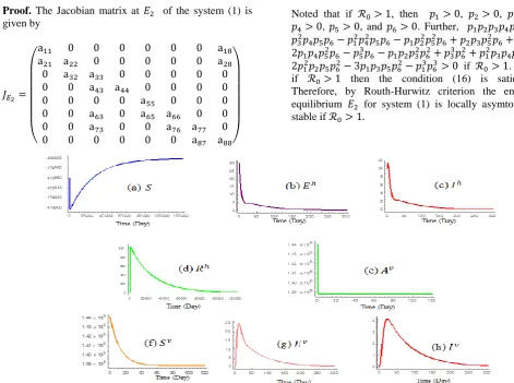
Figure 2: Dynamics of human populations and the population dynamics of mosquitoes for the disease-free equilibrium

IV.

NUMERICAL SIMULATION

Simulations were to justify the stability properties of the equilibrium points based on the

205

Copyright © 2018. IJEMR. All Rights Reserved.

, , ,

and .

4.1 The population dynamics of human and mosquito for the disease-free equilibrium

The parameters used in this simulation for the disease-free equilibrium were , ,

, , , ,

, , , , , , , , ,

(taken from [8] and [12] ). Based on the parameters, we acquired the basic reproduction number

and the disease free equilibrium

. The simulation results for the human population and the mosquito population for the disease-free equilibrium.

In Figure 2a it can be seen that the susceptible humans population rapidly decrease in the begining of time simulation, then the population increase with time and finally approaching the disease-free equilibrium. The exposed humans population rapidly decrease in the begining of time simulation, and continuously decrease until to the end of simulation time (Figure 2b). The infected humans and the recovery humans population, rapidly increase in the begining at time simulation, then the population decrease with time and finally approaching the disease-free equilibrium (Figure 2c-2d). The mosquitoes aquatic population in short time decrease in the begining at time

simulation and then approaching the disease-free

equilibrium (Figure 2e). The susceptible mosquitoes initially increase in the begining at time simulation and then approaching the disease-free equilibrium (Figure 2f). The exposed mosquitoes and infected mosquitoes population initially increase, but the population increase with time and finally approaching the disease-free equilibrium (Figure 2g-2h). The results are consistent with Theorem 3.1 that the disease-free equilibrium

is locally asymptotic stable if

4.2 The population dynamics of human and mosquito for the endemic equilibrium

The parameters used in this simulation for the endemic equilibrium were , ,

, , , , ,

, , , , ,

, , , (taken from [8] and [12]). Based on the parameters then acquired the basic reproduction number and the point remains endemic

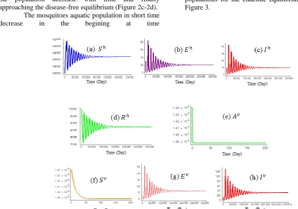
The simulation results for the human and mosquito populations for the endemic equilibrium are shown in Figure 3.

Figure 3: The dynamics of human populations and the population dynamics of mosquitoes for the endemic equilibrium

The susceptible humans population initially increase in short time, then occur fluctuations and finally approaching the endemic equilibrium (Figure 3a). The exposed humans population initially decrease but after

206

Copyright © 2018. IJEMR. All Rights Reserved.

population, the two populations occur fluctuations, then approaching the endemic equilibrium (Figure 3c-3d). The mosquitoes aquatic population in the beginning of simulations decrease until approaching the endemic equilibrium (Figure 3e). Similarly occur to the susceptible mosquitoes population, the susceptible mosquitoes population initially decrease, then approaching the endemic equilibrium (Figure 3f). While the infected mosquitoes and exposed mosquitoes population, initially increased and occur fluctuations, then finally approaching the endemic equilibrium (Figure 3g-3f). The results are consistent with Theorem 3.1 that the endemic equilibrium

is locally asymptotic stable if

4.3 The influence of the number of eggs produced from each compartment per capita

There are three variations of parameter was observed, taken from interval [0-11.2] from [8], and the values of other parameters for the diesease-free equilbrium and the endemic equilibrium is fixed. Figure 4 and 5 shows the effects that occur if the number of eggs produced decreased.

Figure 4: The effect of to the infected humans population, the mosquitoes aquatic and the infected mosquitoes for the diesease-free equilibrium

Figure 5: The effect of to the infected humans population, the mosquitoes aquatic and the infected mosquitoes for the endemic equilibrium

Based on Figure 4a and 5a we can see that decreasing of the number of eggs produced causes the number of the infected humans is on the wane. The same thing occurs to the mosquitoes aquatic (Figure 4b and 5b) and the infected mosquitoes (Figure 4c and 5c). This implies that decreasing of the number of eggs produced helping reduce the rate of spread of dengue disease.

4.4 Effect of the mortality rate from mosquitoes aquatic

There are three variations of parameter was observed taken from interval [0.01-0.47] from [8], and the values of other parameters for the diesease-free equilbrium and the endemic equilibrium is fixed. Figure 6 and 7 shows the effects that occur if the mortality rate of mosquitoes increased.

Figure 6: The effect of to the infected humans population, the mosquitoes aquatic and the infected mosquitoes for the desease-free equilibrium

207

Copyright © 2018. IJEMR. All Rights Reserved.

Based on Figure 6a we can see that increasing of the mortality rate from mosquitoes aquatic causes the number of the infected humans for the diesease-free equilibrium is not too different. While the number of the infected humans for the endemic equilibrium occur change the number of population is decreasing (Figure 7a). The mosquitoes aquatic (Figure 6b and 7b) and the infected mosquitoes (Figure 6c and 7c) population is decreasing. This implies that increasing of the mortality rate from mosquitoes aquatic helping reduce the rate of spread of dengue disease.

V.

CONCLUSION

The mathematical model involving the transmission of dengue disease with aquatic life cycles was considered to describe the transmission of dengue disease. The mathematical model of dengue disease involving aquatic life cycle has two equilibrium points, then namely the disease-free equilibrium and the endemic equilibrium. If the disease-free equilibrium is locally asymptotically stable. The endemic equilibrium is locally asymptotically stable

if . The decrease of and the increase of can

help reduce the rate of disease transmission in the population so that there is no outbreak in the population.

REFERENCES

[1] Tumilaar R, Sian P, & Jaharuddin. (2014). Mathematical models of hemorrhagic disease transmission considering the incubation Period Both Intrinsic and extrinsic. IOSR Journal of Mathematics, 10(5), 13-18.

[2] Stech, H & Williams, M. (2008). Alternate hypothesis on the pathogenesis of dengue hemorrhagic fever (DHF)/dengue shock syndrome (DSS) in dengue virus infection. Experimental Biology Medicine, 233(4), 401-408.

[3] Chung, KW & Lui, R. (2016). Dynamics of two-strain influenza model with cross-immunity and no quarantine class. Journal of Mathematical Biology, 73(6), 1-23.

[4] Tridip, S, Sourav, & R, Joydev, C. (2015). A mathematical model of dengue transmission with memory. Commun. Nonlinear Science and Numerical Simulation, 22, 511-525.

[5] Huang, MG, Tang, MX, & Yu, JS. (2015). Wolbachia infection dynamics by reaction-diffusion equations. Science China Mathematics, 58(1), 77-96. [6] Zheng, B, Tang, MX, Yu, JS. (2014). Modeling Wolbachia spread in mosquitoes through delay differential equations. SIAM Journal of Applied Mathematics, 74(3), 743-770.

[7] Chung, KW & Lui, R. (2016). Dynamics of two-strain influenza model with cross-immunity and no quarantine class. Journal of Mathematical Biology, 73(6), 1-23.

[8] Stech, H & Williams, M. (2008). Alternate hypothesis on the pathogenesis of dengue hemorrhagic fever (DHF)/dengue shock syndrome (DSS) in dengue virus infection. Experimental Biology and Medicine, 233(4), 401-408.