* Corresponding author.
E-mail address: [email protected]
I. Introduction
W
ireless Sensor Network (WSN) consists of independent similar or diverse types of nodes that monitor the environment. These tiny, autonomous, portable and economical nodes sense the data and pass it to designated location or the base station by using wireless ad-hoc network technique. Each sensor node has a transducer, power supply, microcomputer and transceiver to record and process the sensory data [1]. WSN is being used for many applications like industrial process monitoring, battlefield, forest fire detectors, natural disaster prevention, traffic monitoring, etc. [2]. Most of the applications need location information of the sensor nodes for tracking and monitoring [3].In WSN, sensor nodes sense and report the events of interest which can be examined when the position of target nodes reporting the event is known. The information gathered at sink node will be in vain without localization information of sensor nodes. The estimation of the position of sensor nodes is one of the important issues of the WSN and is known as localization problem [4]. Localization can be defined as determining the coordinates of unknown nodes called as target nodes using the position of known nodes called as anchor nodes or beacons [5] based on the measurements such as Time of arrival (TOA), Time difference of arrival (TDOA), Angle of arrival measurement (AOA), etc. [6]. The localization issue can be resolved by deploying each node with Global Positioning System (GPS) but this is not preferred due to size, cost and power factors [7]. Moreover, GPS has restricted functionality as it cannot work indoor and underwater. So, an efficient alternative is required for the localization. The non-GPS based localization algorithms can be used which is categorized into range based and
range free algorithms. Range based localization algorithms uses point to point distance estimation or angle based estimation between sensor nodes whereas range free localization algorithms do not require range information between target node and anchor node but depends on the topological information. The former provides more accuracy as compared to range free localization algorithms.
The range based localization of nodes has two phases – ranging phase and position estimation phase. In the ranging phase, each target node measures its distance from the anchor nodes using the strength of received signal or the signal propagation time. Accurate measurement of distance is not possible due to noise. There is a noisy range measurement irrespective of the ranging method used whereas in position estimation phase, the information acquired from ranging phase is used to determine position of target node. It can also be estimated using geometric approach or by using an optimization algorithm.
The optimization algorithms are really effective in solving NP-Hard problems like Traveling salesman problem, decision subset sum problem, localization, etc. Localization problem is considered as an optimization problem due to size and complexity factors. The analytical methods of optimization like linear programming takes more computation time for solving optimization problems and increase the complexity as the size of problem increases [8]. This propelled to use nature inspired optimization algorithms for WSN as these are robust and effective [9]. These algorithms became popular from the last decade as they can easily adjust to frequently changing environment and have high efficiency [10]. The various algorithms like Particle Swarm Optimization (PSO) [11], Firefly Algorithm (FA) [12] [13], Genetic Algorithm (GA) [14], Grey Wolf Optimization (GWO) [15], Flower pollination Algorithm [16], etc. have been used to determine positions of target nodes. The objective of the various optimization algorithms in WSN localization is to minimize the position estimation DOI: 10.9781/ijimai.2017.03.009
Keywords
Wireless Sensor Network, Localization, Flower Pollination Algorithm, Particle Swarm Optimization, Firefly Algorithm, Grey Wolf Optimization.Abstract
Localization is one of the most important factors highly desirable for the performance of Wireless Sensor Network (WSN). Localization can be stated as the estimation of the location of the sensor nodes in sensor network. In the applications of WSN, the data gathered at sink node will be meaningless without localization information of the nodes. Due to size and complexity factors of the localization problem, it can be formulated as an optimization problem and thus can be approached with optimization algorithms. In this paper, the nature inspired algorithms are used and analyzed for an optimal estimation of the location of sensor nodes. The performance of the nature inspired algorithms viz. Flower pollination algorithm (FPA), Firefly algorithm (FA), Grey Wolf Optimization (GWO) and Particle Swarm Optimization (PSO) for localization in WSN is analyzed in terms of localization accuracy, number of localized nodes and computing time. The comparative analysis has shown that FPA is more proficient in determining the coordinates of nodes by minimizing the localization error as compared to FA, PSO and GWO.
Nature Inspired Range Based Wireless Sensor Node
Localization Algorithms
Ranjit Kaur*, Sankalap Arora
DAV University, Jalandhar, Punjab (India)
error. These nature inspired algorithms really performed well on benchmark functions and localization problem [17]. The work on FPA based node localization algorithm [18] does not provide comparison of two or more localization algorithms with FPA. The distance between target node and an estimated node for each target node has not been reported. In order to provide a fair comparison, it is necessary to show the behavior of the aforementioned techniques considering other values of the parameters involved in the considered algorithms which has not been done yet.
In this paper, the application of FPA, PSO, FA and GWO for the optimal location estimation of sensor nodes is analysed. All the aforementioned factors are considered for the comparison and analysis. These range based localization algorithms are compared with each other to determine the proficient algorithm which performs better to solve localization issue. Factors like transmission range, number of anchor nodes and number of iterations affecting the localization error are considered and analysed for each localization algorithm and compared graphically. All the localization algorithms are analysed in 36 trail runs by changing number of anchor nodes and target nodes in sensor field in terms of localized nodes, localization accuracy and computation time.
The organization of the rest of the paper is as follows: Section II includes literature survey on WSN. Section III describes the meta-heuristic optimization algorithms. Section IV present the localization based on optimization algorithms. In section V, simulation results and comparative study are given and discussed. In section 6, a conclusion along with the future work is presented.
II. Related Work
Localization has become an active research topic in WSN in recent years as exact localization information is really desirable for the performance of WSN. This problem is approached with different methods by the researchers. The localization with Ad-hoc Positioning System (APS)-distributed method in an ad-hoc network is developed by Niculescu [19]. The principle of APS is similar to the GPS but it extends the potential of GPS to non-GPS sensor nodes as position information of anchor nodes is passed to all sensor nodes in the wireless network. For each target node, minimum three anchor nodes are necessary to execute the triangulation or trilateration to determine its location. Another algorithm was proposed by Savarese [20] to improve Niculescu’s method which consists of two phases-hop terrain and refinement. Hop terrain phase is similar to the APS. The refinement phase uses an iterative procedure for the accuracy of location of each node which is enhanced by estimating the least square distances from the neighbouring sensor nodes [21]. The sensor nodes in the sensor field work collectively to determine the location but the error is accumulated in the network. To avoid the accumulation, the kalman filter along with the least square estimation method is used to estimate the co-ordinates of location simultaneously as proposed by Savvides [22]. Localization problem is approached with the convex optimization which is based on semi-definite programming [23]. The technique of semi-definite program is extended further to non- convex inequality constraints by Prtaik [24]. Tzu-Chen Liang extends the Pratik’s method to apply gradient search method [25]. It uses technique of data analysis called multidimensional scaling (MDS) [26]. The range based anchor less localization algorithms are discussed in [27-29].
The localization problem can be considered as an optimization problem. The optimization methods use population based stochastic method to evaluate the location of nodes by minimizing the mean square error [30]. Simulated annealing method was proposed to locate the position of nodes but this doesn’t provide good results. An improved simulated annealing method was proposed which has two
phases. In first phase, the location of target node is estimated whereas in second phase, the optimization is executed on those nodes that may have flip ambiguity problem [31]. The localization algorithms based on GA are proposed in [14], [32], [33]. To minimize the localization error, localization algorithm based on PSO is proposed [30]. The Biogeography Based optimization (BBO) and H-best particle swarm optimization (HPSO) performs better in terms of accuracy and localized nodes as described in [34]. FPA based localization is also proposed to solve the localization issue [18].
III. Nature Inspired Algorithms
Nature inspired algorithms mimics’ nature to solve various hard and complex problems as nature exhibits flexible, robust, diverse and dynamic phenomenon. The nature inspired becomes popular as it can easily adjust to frequently changed environment and the conventional or traditional methods were inefficient. These optimization algorithms really perform well to solve the optimization problems like localization issue, traveling salesman problem, etc. The various algorithms like PSO, FA, FPA, GWO and GA. have been applied to solve the localization problem in WSN. The algorithms which are used for the analysis and comparison are:
A. Flower Pollination Algorithm
FPA is a nature inspired algorithm proposed by Xin-She Yang in 2012 [35]. It is inspired from the natural process ‘pollination of flowers’. This metaheuristic algorithm has evolutionary characteristics and its convergence rate is relatively high as compared to other nature inspired algorithms [36].
Pollination is an intriguing process in which pollen grains are transferred from the anther to the stigma with the help of pollinators for reproduction. It has two major types: biotic and abiotic pollination. Biotic requires help of some living organisms like insects, bats etc. to transfer pollen grains whereas the latter are dependent on wind and water for pollination. There is a process known as flower constancy in which some pollinators visit specific species of flowers bypassing others.
Pollination can be attained by two ways i.e. self-pollination and cross-pollination. Self-pollination is defined as the reproduction of flower by the transfer of pollen grains from the same or different flower of the same plant species whereas in cross-pollination, pollinators like birds, bees, bats etc. travel a long distance for pollination and follows Levy flight behaviour in which the step length obeys Levy distribution.
There are four rules which have been derived for FPA based on the characteristics of pollination which are:
1. Global pollination process is attained by considering biotic and cross pollination because various pollinators performs levy flights. 2. Local pollination is attained through abiotic and self- pollination. 3. Flower constancy is defined as the probability of reproduction
which directly depends on the similarity of two flowers which are involved.
4. Switch probability p ∈ [0, 1] helps in controlling local pollination (exploitation) and global pollination (exploration). In overall pollination activities, local pollination can have a value of p in significant fraction due to the various factors like physical proximity, wind etc.
The first and third rule can be mathematically represented in Eq. (1). ∗)
(1)
Here is pollen i at iteration t or solution vector and ∗ is the global best value in every generation. L is the most important parameter for pollination as the various insects use Levy flight to move over a long distance for pollination [38]. Thus, we draw L > 0 from levy distribution which is valid for large steps i.e. s > 0 [39] and it can be represented as:
)
, (s > 0)
(2)
The local pollination takes place by the transfer of pollen grains with the help of abiotic pollinators from one flower to another. The second rule and flower constancy can be represented mathematically as:)
(3)
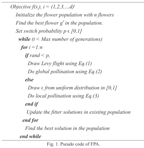
where e and are pollens from distinct flowers of the same plant species at iteration t. It imitates the flower constancy in restricted neighbourhood which helps to attain convergence quickly. If and are from same population and ∈ is drawn from a uniform distribution [0, 1], then it becomes a local random walk. Switch probability p helps to switch from local to global pollination and vice-versa. The pseudo code of the FPA is given in Fig. 1.
Objective f(xi), i = (1,2,3,…d)t
Initialize the flower population with n flowers Find the best flower g* in the population. Set switch probability p ϵ [0,1]
while (t < Max number of generations) for i =1:n
if rand < p,
Draw Levy flight using Eq.(1) Do global pollination using Eq.(2) else
Draw ϵ from uniform distribution in [0,1] Do local pollination using Eq.(3)
end if
Update the fitter solutions in existing population
end for
Find the best solution in the population
end while
Fig. 1. Pseudo code of FPA.
B. Firefly Algorithm
FA was proposed by Xin she Yang in 2009 and it was mainly inspired from the flashing qualities or characteristics of fireflies [40]. The fireflies get attracted to each other despite of their sex. Attractiveness between fireflies depends directly on the brightness due to which less luminous fireflies will be attracted towards brighter firefly. But attractiveness decreases with an increase in distance between them [41]. If there is no brighter firefly available, then firefly will move randomly in the search space. The brightness of the firefly is evaluated by the objective function which is to be optimized [42]. The brightness determines the attractiveness between fireflies corresponding to the objective function. FA is mainly based on two important factors i.e.
change in light intensity and formulation of attractiveness [43]. The intensity of light I changes with distance r having a constant light absorption coefficient which is described mathematically as follows:
(4)
Here Iorepresents light intensity at initial value. The attractiveness between fireflies is relative which is seen or judged by fireflies and it varies with distance r between two fireflies. Thus, the attractivenessβ is defined as follows which is corresponding to the light intensity judged or seen by fireflies.
(5)
Here the represents attractiveness between fireflies when distance r is 0. The Cartesian distance method is used to calculate distance between two fireflies. The firefly i move towards the brighter firefly j which is determined with the help of Eq. (6).
(6)
The second part of the equation represents the attractiveness and the third part is for randomization where the parameter α lies in the range of [0, 1] which helps in randomization and is a random variable whose value is drawn from Gaussian distribution. The pseudo code for this algorithm is given in Fig. 2.
Objective f(xi), i = (1,2,3,…d)t
Initialize the population of fireflies xi (i=1,2,3…n) Set light absorption coefficient γ
While (t < Max number of generations)
for i =1: n fireflies for j =1: n fireflies
Light intensity I_iat x_i is determined by f(xi) if (Ii>Ij)
Move firefly i towards j in d dimensions. end if
Attractiveness changes with distance r using exp[-γr] Evaluate new solutions and update the light intensity
end for j end for i
Rank the fireflies according to light intensity and determine the best firefly
end while
Fig. 2. Pseudo code of FA.
C. Particle Swarm Optimization
The PSO algorithm was proposed by Kennedy and Eberhart [44]. This algorithm is mainly inspired from the behaviour of birds flocking in nature. The flock of birds communicate with each other while migrating to the destination and find the bird at best position. Each bird in the flock moves towards best position with velocity dependent on the current position of the bird and then, they explore the search space from their new positions. The process is reiterated until they reach their destination [45].
( ) and their velocity ( ). The objective function helps to find out the best particle’s position ( ). Every particle in the flock updates their velocity with respect to best particle using following mathematical formula given in Eq. (7).
( ) ∗ ( ) ∗
)
(7)
Here rand ( ) and Rand ( ) are two random functions whose value lies in the range [0, 1]. The and parameters are acceleration constants or learning factors and w represents inertia weight which is mainly used to control the impact of previous velocities of particle on current velocity. The second part of the equation is used to compare the particle’s current position to its own local best position whereas third part compares the particle’s position to the global best particle. The position of a particle using new velocity is updated with the help of Eq. (8).
(8)
The value of lies in the range of user specified values of Vmax, i.e.,
l h to control the effect of change in particle’s velocity. The pseudo code of PSO algorithm is given in Fig. 3.
Objective f(xi), i = (1,2,3,…d)t Initialize the population of particles Initialize the value of inertia weight w
While (t < Max number of generations)
for i: n particles
find local best (pbest) of all particles
end for
find global best (gbest) as the best fitness of all particles
for i: n particles
Calculate the velocity of particle using Eq. (7) Update the position of particle using Eq. (8)
end for end While
Fig. 3. Pseudo code of PSO.
D. Grey Wolf Optimization
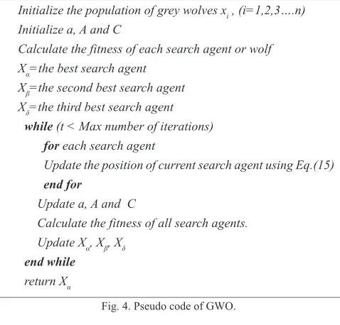
Grey Wolf Optimizer (GWO) is a nature inspired algorithm proposed by Mirjalili et al. in 2014 that focuses on social behaviour of grey wolves [47]. This algorithm is inspired from grey wolves that belong to canidae family. It simulates the leadership quality and the hunting behaviour of grey wolves in three steps as tracking, encircling and attacking. Grey wolves consists of 5-12 wolves. Grey wolves live in pack that contains 5-12 wolves. α, β, δ and ω are four types of grey wolves following a strict social hierarchy. α is the dominant wolf among the other grey wolves that makes different decisions which are followed by other submissive grey wolves. β grey wolf is second in the hierarchy after α grey wolf. β grey wolf help the dominant leader α to make decisions about sleeping etc.
Approaching and encircling the prey are behaviour of team hunting followed by the grey wolves’ pack which is mathematically modelled in Eq. (9) and Eq. (10).
( ) ( )
(9)
( ) ( )
(10)
Here and represents the position vector of grey wolf and prey. Vectors and are depicted with the help of following equations:
(11)
(12)
Here Here and are random vectors in range [0, 1] and parameter r is linearly decreased from 2 to 0. The best three solutions are saved and further the candidate solutions i.e., grey wolves update their positions accordingly. Social behavior of hunting mechanism is mathematically derived using Eq. (13), (14) and Eq. (15).
,
,
(13)
( ) . ( ),
( ) ,
( ) . ( )
(14)
( ) =
(15)
At the end, when the last criterion specified will be satisfied, GWO algorithm will get terminated and the best position of α wolf will be considered as the outcome. All the steps are presented in pseudo code which is given in Fig. 4.
Initialize the population of grey wolves xi , (i=1,2,3….n) Initialize a, A and C
Calculate the fitness of each search agent or wolf Xα=the best search agent
Xβ=the second best search agent Xδ=the third best search agent
while (t < Max number of iterations)
for each search agent
Update the position of current search agent using Eq.(15)
end for
Update a, A and C
Calculate the fitness of all search agents. Update Xα, Xβ, Xδ
end while
return Xα
Fig. 4. Pseudo code of GWO.
nature inspired algorithm is shown in Fig. (5).
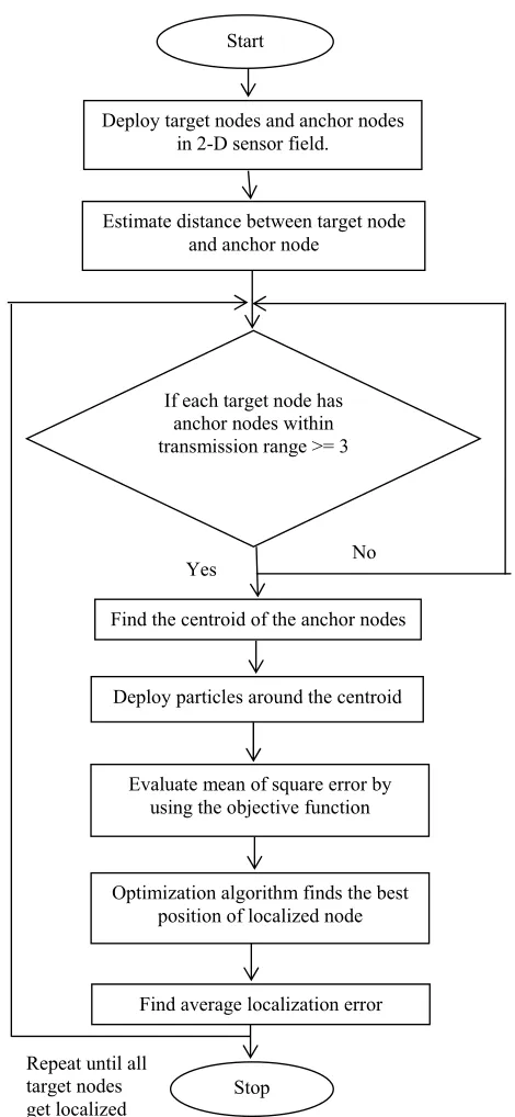
The following steps are followed to perform node localization of each target node in WSN:
1. M target nodes and N beacons or anchor nodes are deployed randomly in the sensor field. Each anchor node has transmission range R. The localized nodes act as beacon in next iteration to remove flip ambiguity problem.
Start
Deploy target nodes and anchor nodes in 2-D sensor field.
Estimate distance between target node and anchor node
If each target node has anchor nodes within transmission range >= 3
Find the centroid of the anchor nodes
Deploy particles around the centroid
Evaluate mean of square error by using the objective function
Optimization algorithm finds the best position of localized node
Find average localization error
Stop
No Yes
Repeat until all target nodes get localized
Fig. 5. Flow chart of Sensor node localization using nature inspired algorithm.
2. The distance between each target node and anchor node is measured. There is an additive white Gaussian noise which blurs the measurement. Each target node’s distance from every anchor node is measured as where is the actual distance and is the measurement noise which has gaussian distributed random value in the range ( ) which really affects the
performance of the localization algorithm as the localization error increases with the increase in noise. The actual distance can be measured by using the Eq. (16):
= ) )
(16)
Where (x, y) and ( , ) are the coordinates of target node and anchor node respectively.
3. The target node that has anchor node ≥ 3 within its transmission range is known as localizable node. This target node is localized using an optimization algorithm.
4. For each target node, an optimization algorithm is executed independently. Initialize the particles of the algorithm with the centroid of the anchor nodes (within the transmission range) by using the Eq. (17) as follows:
(x , y ) ∑ x , ∑ y
(17)
where N is the number of the anchor nodes within transmission range of each target node.
5. The algorithm minimizes the objective function or error for the localization problem in WSN which is given mathematically in Eq. (18).
( ) = (∑ ( ) + ( ) )
(18)
where N ≥3 are the number of anchor nodes within transmission range, ) is the anchor node within the transmission range and
(x,y) is the position of the particles.
6. FPA finds the optimal value (X, Y) after the maximum number of iterations.
7. When the position of all localized nodes get estimated, compute the average localization error to find the localization accuracy by using the Eq. (19) as follows:
= ∑ ) )
(19)
where ) are the coordinates of actual node, ( , ) are the coordinates of estimated position and is the total number of localized nodes.
8. Repeat steps 2-7 until all the target nodes get localized or no more target nodes can be localized. The localization algorithm’s performance is based on the estimated average localization error and the number of un-localized nodes where = M− . Localization accuracy is better if value of and is less. The number of localized nodes increases as the iteration increments. A node that has been localized can be used as a beacon for the next node. This decreases the problem of flip ambiguity as more references are available for the localized node. However, this increases the computation time.
V. Simulation Results and Discussion
algorithms in terms of localized node ( ), localization error ( ) and computation time (( ). The parameter values that provide better localization accuracy are considered for the localization algorithms. The strategic settings and parameter values of PSO, FA, GWO and FPA are discussed below:
A. PSO Based Localization
The performance of PSO based localization with different parameters is analysed and summarized in Table 1. The parameter values that result in less localization error are considered. The inertia weight is an important parameter to control the effect of the previous velocities on the existing velocity and the parameters and is the learning factors. The number of particles n helps to localize a target node by updating the position according to optimization algorithm. The number of iterations represents the number of times the position is updated to find an optimal solution. The parameter values that works best for localization is considered for PSO based node localization algorithm which are as follows.
• No. of particles or population (n) = 30 • No. of iterations = 100
• Cognitive or social scaling parameter = = 1.494 • Inertia weight (w) = 0.7
TABLE I. Performance of PSO with Different Tuning Parameters
S. No. Parameters
1. w 0.7 100 0.584384 2.287
0.4 100 0.650246 2.206
2. = 1.494 100 0.690518 2.259
2.0 100 0.694749 2.45
3. n 20 100 0.721967 2.21
30 100 0.717235 1.997
4. iteration 100 100 0.698956 2.591
200 100 0.567573 4.335
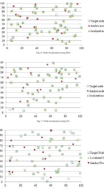
The PSO based localization algorithm is conducted using above parameters for specified number of iterations to find the localization information. The localized nodes, 50 target nodes and 15 anchor nodes are depicted in Fig. 6.
B. FA Based Localization
Each localized node runs FA to estimate the position of sensor nodes in the sensor field. The performance of FA based localization is evaluated by tuning parameters and summarized in Table 2. The parameter γ is the light absorption coefficient which is really important for the convergence of the algorithm. The value of randomization factor
α lies between [0, 1] and β is the initial attractiveness when the distance between two fireflies is 0. The value of n shows the number of fireflies to be deployed in the sensor field to attain the localization information by running the algorithm for specified number of iterations.
The parameters which shows less localization error are considered for localization which are:
• No. of fireflies (n) = 30 • No. of iterations = 100
• Randomization parameter (α) = 0.25 • Absorption coefficient (γ) = 1.0 • Initial attractiveness (β) = 1.0
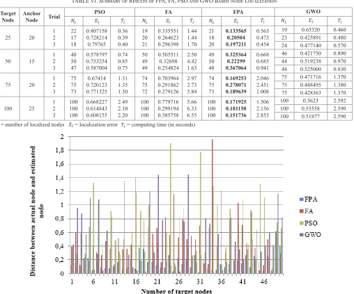
FA is run for each target node till the specified number of iterations to localize target nodes. FA based localization for 50 target nodes is represented in Fig.7
TABLE II. Performance of FA with Different Tuning Parameters
S. No. Parameters
1. α 0.25 100 0.903181 6.503
0.50 100 1.01864 8.737
2. β 1.0 100 0.528133 7.892
0.2 100 0.378845 9.133
3. γ 1.0 100 0.410389 7.618
0.7 100 0.430746 7.743
4. n 20 100 0.360542 5.229
30 100 0.366548 6.763
5. Iteration 100 100 0.305937 8.681
200 100 0.576672 9.315
C. GWO Based Node Localization
The performance of GWO based node localization algorithm considering the parameters is summarized in Table 3. The vector is a controlling parameter for exploration and exploitation in an algorithm which linearly decreases from 2 to 0. The numbers of grey wolves or particles n helps to determine the localization information of target node by updating their position.
The following parameters are considered for the localization of target nodes using GWO:
• No. of particles (n) = 30 • No. of iterations = 100 • vector = 2 to 0
TABLE III. Performance of GWO with Different Tuning Parameters
S. No. Parameters
1. 2 to 0 100 0.382065 2.894
2. n 20 100 0.442893 2.531
30 100 0.362075 2.734
3. iteration 100 100 0.445948 2.531
200 100 0.314762 2.406
GWO based node localization of 50 target nodes with 15 anchor nodes is illustrated in Fig. 8 which shows target nodes, localized nodes and anchor nodes.
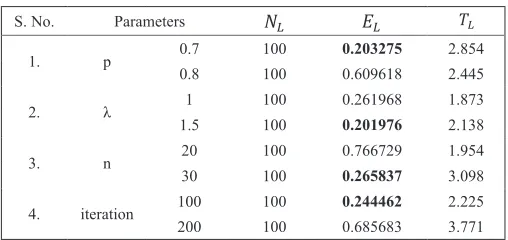
D. FPA Based Node Localization
The performance of the FPA based localization algorithm is analysed and summarized by considering parameters in Table 4.
Table IV. Performance of FPA with Different Tuning Parameters
S. No. Parameters
1. p 0.7 100 0.203275 2.854
0.8 100 0.609618 2.445
2. λ 1 100 0.261968 1.873
1.5 100 0.201976 2.138
3. n 20 100 0.766729 1.954
30 100 0.265837 3.098
4. iteration 100 100 0.244462 2.225
Fig. 6. Node localization using PSO.
Fig. 7. Node localization using FA.
The parameter switch probability p is mainly used to control the global pollination and local pollination of the algorithm. The value of
λ is really crucial for the Levy flight which plays an important role for global pollination. The number of pollens n is deployed around the centroid of the anchor nodes which update the position with the help of position updating formulas for specified number of times. The following parameters are considered for FPA based localization algorithm:
• No of pollen/flowers (n) = 30 • No. of iterations = 100 • Switch probability (p) = 0.7 • Lambda (λ) = 1.5
50 target nodes estimated by FPA based node localization with the help of 15 anchor nodes is depicted in Fig.9.
The nature inspired optimization algorithms are stochastic in nature. So, same results are not produced in all runs or experiments. Due to this, the results of 30 trial experiments are averaged by using = 2,
M = 50 and N = 15. The results are summarized in Table 5 which shows that FPA performs better with respect of localization error and un-localized node. The computation time taken by PSO is less than other algorithms. GWO performs less among other algorithms in terms of localization error.
Table V. Summary of Results of 30 Trial Runs
Algorithms Mean Mean Computing time (s)
FPA 4.5 0.28374 0.767
PSO 7.1 0.584231 0.743
FA 5.4 0.725323 3.891
GWO 5.0 0.802848 0.832
The initial deployment of sensor nodes is random due to which the localization accuracy, the number of un-localized node and the total computing time will be different for every run of the localization algorithm. The beacons, target node and the position estimated by the algorithms like PSO, FA, GWO and FPA are shown in Fig. 6, 7, 8 and 9 respectively
The transmission range, additive Gaussian noise and the number of anchor nodes are the important parameters to determine the localization error. The performance of localization algorithms is influenced by these parameters. Dependency of the percentage of the localized node on the number of anchor nodes for FA, PSO, GWO and FA based localization algorithms is shown in Fig. 10. The performance of the localization
algorithm depends on the density of anchor nodes. It is difficult to locate position of nodes if sufficient number of anchor nodes (N >= 3) are not available. The less number of anchor nodes localize very few number of target nodes. Location estimation accuracy and the percentage of localized nodes increase with the increase in anchor node density. The increase in transmission range of anchor nodes helps in improving the performance as the number of anchor nodes within transmission range of each target node will be more. This will also increase the number of localized nodes. The dependency of localized nodes on the transmission range for FA, PSO, GWO and FPA is shown in Fig. 11. Smaller transmission range localizes very less number of sensor nodes.
Fig. 10. Percentage of localized nodes depending on the number of anchor nodes
Gaussian additive noise is also an important parameter that has a great impact on localization accuracy. As noise in distance measurement increases, increases which leads to decrease in localization accuracy. Due to this, all the experiments are conducted by considering Gaussian noise = 2.
The localization accuracy also improves with the increase in number of iterations as shown in Fig. 12. As the number of iteration progresses, the localization error declines. FPA shows more decline in the error as compared to other two algorithms.
The distance between target node and estimated node for varying number of target nodes is shown in Fig. 13. In this estimated distance for each target node using optimization algorithms is compared which shows FPA based node localization performs better for target nodes which shows its proficiency. Node localization based on FA, PSO, GWO and FPA algorithms by varying number of anchor and target nodes is summarized in Table 6. All the experiments are conducted with different configurations in 36 trails. All the optimization algorithms performed well to estimate the location of nodes in WSN. The FPA based localization algorithms provides less localization error for each number of target nodes whereas PSO estimate the position in less computing time but it has high localization error. It shows
better localization accuracy to estimate the position than FA, PSO and GWO localization algorithms in terms of mean square error. But the computing time required by FPA in locating the sensor nodes is more than other optimization algorithms. However, the performance of GWO is comparative less to other algorithms like FA, PSO and FPA in terms of localization accuracy and computation time.
Fig. 13. Distance between actual node and estimated node with different optimization algorithms. TABLE VI. Summary of Results of FPA, FA, PSO and GWO Based Node Localization
Target
Node Anchor Node Trial
PSO FA FPA GWO
25 20 12
3 22 17 18 0.807158 0.728214 0.79765 0.36 0.39 0.40 19 20 21 0.335551 0.264623 0.296398 1.44 1.44 1.70 21 18 20 0.133565 0.20504 0.197211 0.563 0.473 0.454
19 0.65320 0.460
23 0.425891 0.480
24 0.477140 0.570
50 15 12
3 48 50 47 0.578797 0.753254 0.587004 0.74 0.85 0.75 50 49 49 0.505511 0.32698 0.254824 2.50 4.42 1.63 49 50 48 0.325364 0.22299 0.367064 0.668 0.685 0.941
46 0.421750 0.890
44 0.519238 0.970
48 0.525000 0.830
75 20 12
3 75 75 73 0.67414 0.720123 0.771325 1.31 1.35 1.30 74 75 72 0.703964 0.291862 0.279126 2.97 2.73 3.84 74 75 73 0.169253 0.278071 0.189639 2.046 2.451 1.008
75 0.471716 1.370
75 0.448495 1.380
75 0.428363 1.370
100 25 12
3 100 100 100 0.668227 0.614843 0.608155 2.49 2.10 2.20 100 100 100 0.779716 0.299194 0.385758 5.66 6.33 6.55 100 100 100 0.171925 0.181158 0.151736 1.506 2.156 2.853
100 0.3623 2.592
100 0.55558 2.590
100 0.51877 2.590
= number of localized nodes = localization error = computing time (in seconds)
VI. Conclusion
Localization of sensor nodes is really important for the performance of WSN as many applications of WSN require localization information. The main objective of this optimization problem is to minimize the localization error with the help of nature-inspired optimization algorithms. In this paper, node localization using meta-heuristic optimization algorithm like Firefly Algorithm (FA), Particle Swarm Optimization (PSO) and Grey Wolf Optimization (GWO) algorithm is conducted to determine the position of the sensor nodes in WSN. This paper has analysed the localization problem and solved it with different optimization algorithms and provides the summary of results by comparing the algorithm with the each other in terms of localization error, localized nodes and computing time. The FPA based node localization algorithm shows better localization accuracy in estimating the position than other algorithms. GWO performs comparative less with respect to localization error and computation time among the optimization algorithms. These distributed localization algorithms are better than centralized algorithms as the number of transmissions to the sink node is reduced which helps to conserve the energy of sensor nodes. These localization algorithms further can be implemented for centralized method and can be compared with distributed method for analysis. FPA can be hybridized with other optimization algorithm to further minimize the location estimation error. These optimization algorithms can be implemented in 3D scenario to find localization accuracy. The parameter values can be varied to improve the optimization algorithm to improve convergence rate, localization accuracy and computation time.
References
[1] R. V. Kulkarni, A. Förster, G. K. Venayagamoorthy, Computational
intelligence in wireless sensor networks: a survey, Communications Surveys & Tutorials, IEEE 13 (1) (2011) 68–96.
[2] I. F. Akyildiz,W. Su, Y. Sankarasubramaniam, E. Cayirci, Wireless sensor
networks: a survey, Computer networks 38 (4) (2002) 393–422.
[3] J. Yick, B. Mukherjee, D. Ghosal, Wireless sensor network survey,
Computer networks 52 (12) (2008) 2292–2330.
[4] R. V. Kulkarni, G. K. Venayagamoorthy, Particle swarm optimization in
wireless-sensor networks: A brief survey, Systems, Man, and Cybernetics, Part C: Applications and Reviews, IEEE Transactions on 41 (2) (2011) 262–267.
[5] J.Wang, R. K. Ghosh, S. K. Das, A survey on sensor localization, Journal
of Control Theory and Applications 8 (1) (2010) 2–11.
[6] G. Mao, B. Fidan, B. D. Anderson, Wireless sensor network localization
techniques, Computer networks 51 (10) (2007) 2529–2553.
[7] R. G. Crespo, G. G. Fernandez, O. S. Martínez, V. García-Díaz, L. J.
Aguilar, E. T. Franco, In premises positioning–fuzzy logic, in: International Work-Conference on Artificial Neural Networks, Springer, 2009, pp. 284– 291.
[8] R. V. Kulkarni, G. K. Venayagamoorthy, Bio-inspired algorithms for
autonomous deployment and localization of sensor nodes, Systems, Man, and Cybernetics, Part C: Applications and Reviews, IEEE Transactions on 40 (6) (2010) 663–675.
[9] R. V. Kulkarni, G. K. Venayagamoorthy, M. X. Cheng, Bioinspired
node localization in wireless sensor networks, in: Systems, Man and Cybernetics, 2009. SMC 2009. IEEE International Conference on, IEEE, 2009, pp. 205–210.
[10] J. Meza, H. Espitia, C. Montenegro, R. G. Crespo, Statistical analysis of a
multi-objective optimization algorithm based on a model of particles with vorticity behavior, Soft Computing (2015) 1–16.
[11] A. Gopakumar, L. Jacob, Localization in wireless sensor networks
using particle swarm optimization, in: Wireless, Mobile and Multimedia Networks, 2008. IET International Conference on, IET, 2008, pp. 227– 230.
[12] R. Harikrishnan, V. J. S. Kumar, P. S. Ponmalar, Firefly algorithm
approach for localization in wireless sensor networks, in: Proceedings of
3rd International Conference on Advanced Computing, Networking and Informatics, Springer, 2016, pp. 209–214.
[13] S. Arora, S. Singh, A conceptual comparison of firefly algorithm, bat
algorithm and cuckoo search, in: Control Computing Communication & Materials (ICCCCM), 2013 International Conference on, IEEE, 2013, pp. 1–4.
[14] Q. Zhang, J. Wang, C. Jin, J. Ye, C. Ma, W. Zhang, Genetic algorithm
based wireless sensor network localization, in: Natural Computation, 2008. ICNC’08. Fourth International Conference on, Vol. 1, IEEE, 2008, pp. 608–613.
[15] M. M. Fouad, A. I. Hafez, A. E. Hassanien, V. Snasel, Grey wolves
optimizer-based localization approach in wsns, in: 2015 11th International Computer Engineering Conference (ICENCO), IEEE, 2015, pp. 256–260.
[16] M. Sharawi, E. Emary, I. A. Saroit, H. El-Mahdy, Flower pollination
optimization algorithm for wireless sensor network lifetime global optimization, International Journal of Soft Computing and Engineering 4 (3) (2014) 54–59.
[17] X.-S. Yang, Nature-inspired metaheuristic algorithms, Luniver press,
2010.
[18] S. Goyal, M. S. Patterh, Flower pollination algorithm based localization f
wireless sensor network, in: 2015 2nd International Conference on Recent Advances in Engineering & Computational Sciences (RAECS), IEEE, 2015, pp. 1–5.
[19] D. Niculescu, B. Nath, Ad hoc positioning system (aps), in: Global
Telecommunications Conference, 2001. GLOBECOM’01. IEEE, Vol. 5, IEEE, 2001, pp. 2926–2931.
[20] C. S. J. Rabaey, K. Langendoen, Robust positioning algorithms for
distributed ad-hoc wireless sensor networks, in: USENIX technical annual conference, 2002, pp. 317–327.
[21] N. Bulusu, D. Estrin, L. Girod, J. Heidemann, Scalable coordination
for wireless sensor networks: self-configuring localization systems, in: International Symposium on Communication Theory and Applications (ISCTA 2001), Ambleside, UK, 2001.
[22] A. Savvides, H. Park, M. B. Srivastava, The bits and flops of the n-hop
multilateration primitive for node localization problems, in: Proceedings of the 1st ACM international workshop on Wireless sensor networks and applications, ACM, 2002, pp.112–121.
[23] L. Doherty, K. S. Pister, L. El Ghaoui, Convex position estimation in
wireless sensor networks, in: INFOCOM 2001. Twentieth Annual Joint Conference of the IEEE Computer and Communications Societies. Proceedings. IEEE, Vol. 3, IEEE, 2001, pp. 1655–1663.
[24] P. Biswas, Y. Ye, Semidefinite programming for ad hoc wireless sensor
network localization, in: Proceedings of the 3rd international symposium on Information processing in sensor networks, ACM, 2004, pp. 46–54.
[25] T.-C. Liang, T.-C. Wang, Y. Ye, A gradient search method to round the
semidefinite programming relaxation solution for ad hoc wireless sensor network localization, Sanford University, formal report 5.
[26] Y. Shang,W. Rum, Improved mds-based localization, in: INFOCOM
2004. Twenty-third Annual Joint Conference of the IEEE Computer and Communications Societies, Vol. 4, IEEE, 2004, pp. 2640–2651.
[27] S. Cˇ apkun, M. Hamdi, J.-P. Hubaux, GPS-free positioning in mobile ad
hoc networks, Cluster Computing 5 (2) (2002) 157–167.
[28] U. Ferner, H. Wymeersch, M. Z. Win, Cooperative anchor-less localization
for large dynamic networks, in: Ultra-Wideband, 2008. ICUWB 2008. IEEE International Conference on, Vol. 2, IEEE, 2008, pp. 181–185.
[29] A. Youssef, A. Agrawala, M. Younis, Accurate anchor-free node
localization in wireless sensor networks, in: Performance, Computing, and Communications Conference, 2005. IPCCC 2005. 24th IEEE International, IEEE, 2005, pp. 465–470.
[30] S. Yun, J. Lee,W. Chung, E. Kim, S. Kim, A soft computing approach to
localization in wireless sensor networks, Expert Systems with Applications 36 (4) (2009) 7552–7561.
[31] A. A. Kannan, G. Mao, B. Vucetic, Simulated annealing based wireless
sensor network localization with flip ambiguity mitigation, in: Vehicular Technology Conference, 2006. VTC 2006-Spring. IEEE 63rd, Vol. 2, IEEE, 2006, pp. 1022–1026.
[32] Q. Zhang, J. Huang, J. Wang, C. Jin, J. Ye, W. Zhang, A new centralized
[33] Q. Zhang, J. Wang, C. Jin, Q. Zeng, Localization algorithm for wireless sensor network based on genetic simulated annealing algorithm, in: Wireless Communications, Networking and Mobile Computing, 2008. WiCOM’08. 4th International Conference on, IEEE, 2008, pp. 1–5.
[34] A. Kumar, A. Khosla, J. S. Saini, S. Singh, Meta-heuristic range based
node localization algorithm for wireless sensor networks, in: Localization and GNSS (ICL-GNSS), 2012 International Conference on, IEEE, 2012, pp. 1–7.
[35] X.-S. Yang, Flower pollination algorithm for global optimization, in:
Unconventional computation and natural computation, Springer, 2012, pp. 240–249.
[36] X.-S. Yang, M. Karamanoglu, X. He, Flower pollination algorithm: a
novel approach for multiobjective optimization, Engineering Optimization 46 (9) (2014) 1222–1237.
[37] X.-S. Yang, Nature-inspired optimization algorithms, Elsevier, 2014.
[38] S. Arora, S. Singh, Butterfly algorithm with levy flights for global
optimization, in: Signal Processing, Computing and Control (ISPCC), 2015 International Conference on, IEEE, 2015, pp. 220–224.
[39] I. Pavlyukevich, L´evy flights, non-local search and simulated annealing,
Journal of Computational Physics 226 (2) (2007) 1830–1844.
[40] X.-S. Yang, Firefly algorithm, stochastic test functions and design
optimisation, International Journal of Bio-Inspired Computation 2 (2) (2010) 78–84.
[41] S. Arora, S. Singh, S. Singh, B. Sharma, Mutated firefly algorithm,
in: Parallel, Distributed and Grid Computing (PDGC), International Conference on, IEEE, 2014, pp. 33–38.
[42] S. Arora, S. Singh, Performance research on firefly optimization algorithm
with mutation, in: International Conference, Computing & Systems, 2014.
[43] S. Gupta, S. Arora, A hybrid firefly algorithm and social spider algorithm
for multimodal function, in: Intelligent Systems Technologies and Applications, Springer, 2016, pp. 17–30.
[44] R. C. Eberhart, J. Kennedy, et al., A new optimizer using particle swarm
theory, in: Proceedings of the sixth international symposium on micro machine and human science, Vol. 1, New York, NY, 1995, pp. 39–43.
[45] J. Meza, H. Espitia, C. Montenegro, E. Giménez, R. González- Crespo,
Movpso: Vortex multi-objective particle swarm optimization, Applied Soft Computing.
[46] Y. Shi, R. C. Eberhart, Empirical study of particle swarm, in: Evolutionary
Computation, 1999. CEC 99. Proceedings of the 1999 Congress on, Vol. 3, IEEE, 1999.
[47] S. Mirjalili, S. M. Mirjalili, A. Lewis, Grey wolf optimizer, Advances in
Engineering Software 69 (2014) 46–61.
Ranjit Kaur
Ranjit Kaur received M.Tech in computer science and engineering from DAV University, Jalandhar, Punjab (India) and B.Tech in Computer Science Engineering from Punjab Technical University, Jalandhar, Punjab (India). Her current research interests includes optimization, nature inspired algorithms and wireless sensor networks.
Sankalap Arora