An evaluation of Cyclotron Effective Mass and Electron g-factor in Semiconductor Quantum Well

An evaluation of Cyclotron Effective Mass and Electron

g-factor in Semiconductor Quantum Well

TAJENDRA KAUR1, A. K. SINHA2, H.S.SINGH3, S. KUMAR4 and L. K. MISHRA

Department of Physics,

Magadh University, Bodh-Gaya, INDIA. 1

Research Scholar, Bauliya, Salimpur Ahra, Exhibition Raod, Patna, INDIA. 2

Department of Physics, B.D. College, Patna, INDIA.

3

Department of Physics, J. D.Women’s College, Patna, INDIA. 4

Magadh Colony, Road No.-12/B, Chandauti, Gaya, INDIA. (Received on: February 9, 2013)

ABSTRACT

Using the theoretical formalism of M. De Dios-Leyva et al. (2006), we have evaluated the cyclotron effective mass, 2D cyclotron effective mass and g11-factor for GaAs-Ga0.65Al0.35AS

quantum well both as a function of magnetic field B (T) and also as a function of well width (A˚). Our theoretical evaluated results are in good agreement with the experimental data.

Keywords: Cyclotron effective mass g -factor, Semiconductor quantum well, effective mass approximation, Landau states.

1. INTRODUCTION

The understanding of the physics of wells (QWs), and quantum well wires (QWWs), Quantum dots (QDs) and super lattices (SLs) has been a great interest to solid state physics, several studies have been performed to evaluate the physical properties of these systems1-6. The possible use of electron spins in the architecture of solid state based quantum computer has

and also in the interpretation of experimental date in this research. These factors play an important role in the magneto-optical and magneto-transport studies optically detected nuclear response experiments, spin electronic and quantum beats measurements. These are also applied the integer quantum Hall Effect.

For the calculation of electron g-factor and cyclotron effective mass one needs the detailed understanding of the interaction between the external applied magnetic field and the electronic state of semiconductor hetrostructure. One new technique like electron spin resonance, spin quantum beats, spin Raman scattering experiments and capacitance and energy spectroscopic. Lattice effects on the orbital contribution, quantum confinement and applications of hydrostatic pressure and external electric/magnetic field may considerably modify conduction electron g-factor both in magnitude and sign in different semiconductor hetrostructure. Theoretical point of view both electron g-factor and cyclotron effective mass provide an excellent tool for testing the band structure electronic calculation in the dimensional semiconductor hetrostructure.

In this paper, we have evaluated cyclotron effective mass (Mc/Mo) and 2D cyclotron effective mass (M2D/Mo) as a function of magnetic field B (T). We have also evaluated (mc/mo) and g11 factor as a function of well width (A0) for GaAs and Ga0.65Al0.35As QW keeping (L=50A0). Our theoretical evaluated results are in good agreement with the experimental data.

2. MATHEMATICAL FORMULA USED IN THE EVALUATION

One uses Ogg-McCombe

Hamiltonian 11-18 within the effective mass approximation and in the forth order of

k p

.

perturbation theory. This Hamiltonian acts on the two fold Γ6 spin degenerate conduction band of the bulk materials of the GaAs-Ga1-xAl As quantum well under an applied magnetic field parallel in the growth z-direction. This is written as

2

4 1 *

1

.

2 2 B z

H K I g B a K I

m µ σ σ τ

= h uur r+ + Γ + uuurr+

(1)

2 2 2 2

2

3 4

4 [{ x, y } { y, z}] z B

a

I a k k k k I a B

l + + +

σ

r r

+a5{ . ,

σ

K k BIz }+a B6

σ

zk2z+V z I( )

r r

Where ܫҧ is the 2x2 unit matrix

ˆ ˆ

ˆ

/

K = +k eA c

r r

r

h

ˆ

K = − ∇i

r

Landau gauge is used for the vector potential

ˆ

ˆ

A

= −

yBx

r

r

ai = 1-6 are constants taken from ref. 14 for equal values for the well and barrier materials.

V(z) is square well confining potential taken from Ga1-x AlxAs and GaAs band gap offset.19

m* and g are the z-growth direction position dependent conducton electron effective mass and Landu g-factor.

Γ is constant associated with spin orbit term (due to the fact that GaAs has no. inversion symmetry), l_B c

eB

µβ is the Bohr magneton

σ

ˆ =(

σ σ σ

ˆx, ˆy, ˆz)is the Pauli matrices and

τ

ˆ

is a vector operator

with components such as

ˆ ˆ ˆ ˆ ˆ ˆ

ˆ_x k k k_{y x y} k k k_{z x z}

τ

= − _{and corresponding}

cyclic permutation. The above Hamiltonian is a 2 x 2 conduction band effective Hamiltonian.13-15 This Hamiltonian includes effects of non-parabolicity by taking into account the coupling between the lowest Г6c conduction band, Г7ν and Г8ν valance bands and the Г7c and Г8c p - anti bonding conduction bands.

The 2nd.term in RHS of eqn. (1) is the Zeeman contribution, the second order in

k

r

spin dependent term (with the factor a4, a5, and a6) together with the third one is spin orbit interaction). The third order k contributes the changes in the hetrostructure effective g-factor. The terms in a1 and a3 govern the energy dependence of the Cyclotron effective mass where as term with a2 gives the diamagnetic shift of the Landau electronic length.

Let the Eigen function of H be

( )

( , )

ikx

x

e

r

y z

L

ψ

=

φ

(2)

Here kx is good quantum number as

ˆ

Hdoes not depend on x explicitly. Lx is QW length along x direction.

ψ

( )xr

and

φ

( , )y z

are two component wave function. Now we write the Hamiltonian20,21

0

ˆ ˆ ˆ

H =H +W (3)

whereWˆ is the perturbed Hamiltonian and may be neglected. This only contributes small correction to the

energy levels.22 The Eigen function of 0

ˆ₍ ˆ ₎

H orH may be written as

(

,

)

1

( )

iK xx

( )

( )

n n m

x

r

e

y f

z

L

ψ

φ

+

+

=

(4)

and 0 1 ( ) ( ) , ( ) x iK x n n x r e

y f m z L

ψ

−

φ

 

=  

  (5)

Where the symbols ± corresponds to (↑) spin up and (↓) spin down states respectively. Eigen functions

φ

_n

( )

y

is 1D harmonic oscillator is given by

2

0 0

1 1 2

2 2

( )

1

( ) ( )

2

[ !2 ]

n n

n B B

B

y y y y

y e H

l l n l φ π − − − = (6) Where Hn are the Hermite polynomials, yo=Kxl_Β is the orbit centre position and En=ћωc(n+1/2) with n=0, 1, 2, ... and ωc=eΒ/m*c are the 1D energies. The sub-index m = 1, 2, 3, ... in both fn,m± (z) and is associated with the electronic levels

,

n m

E± . This indicates ,

n m

E± m-th QW confined energy and n=0, 1, 2, ... for given m represents the corresponding sub bands energy level.24

The Cyclotron effective mass is given by , , 1 / [ ( ) ( )] c n n eB c m

E B E B

↑↓ ↑ ↓ ↑ ↓ + = − h (7)

2 _{, ,}

( / )( 1/ 2)

[ ( ) ( 0)]

D

n n

eB c n m

E B E B

↑↓

↑ ↓ ↑ ↓

+ =

− =

h

(8)

The parallel g-factor is

[

_n

( )

_n

( )]

B

E

B

E

B

g

B

µ

↑

−

↓

=

(9)

3. DISCUSSION OF RESULTS

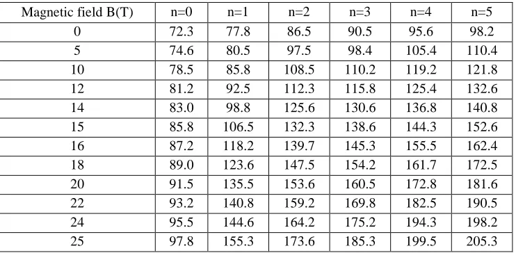
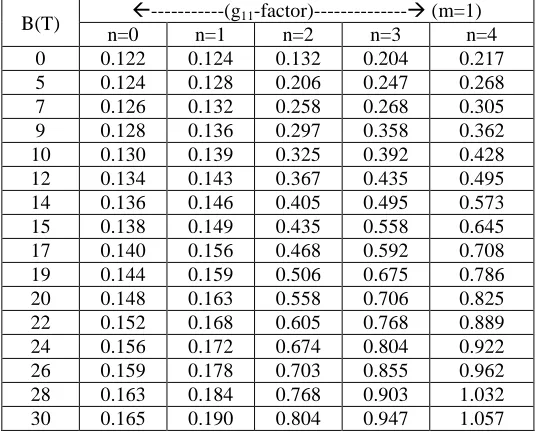
In this paper, using the theoretical formalism developed by M. De. Dios-Leyva et al., 25 we have theoretically evaluated electronic Landau level energy, Cyclotron effective mass (Mc/mo), 2D Cyclotron effective mass (m2D/mo) and g11-factor for L=50Ao GaAs-Ga0.65Al0.35As QW as a function of as a function of the growth direction applied magnetic field. The results are shown in table T1, T2, T3 and T4 respectively. We have also evaluated cyclotron effective mass (mc/mo) for GaAs-Ga0.65Al0.35As QW as a function of well width. The theoretical results were compared with experimental data I25 and II26. The results are shown in table T5. In another evaluation, we have obtained the theoretical result of g11-factor for GaAs-Ga0.65Al0.35As QW as a function of well width (A˚). The results are compared with another two experimental data I27 and II which is shown in table T628.

In table T1, we have shown the electronic levels of the first m=1 sub bands of Landau levels. The non-linear behaviour of the E±_{n m,} =1 Landau electronic levels is due to the presence of non-parabolic terms in the Hamiltonian. Our theoretical result

Table T1

An evaluated results of electronic Landau levels as a function of the growth direction applied magnetic field for L=50Ao, GaAs-Ga0.65Al0.35As Quantum Well for m=1 sub-bands of Landau states.

Magnetic field Β(T) n=0 n=1 n=2 n=3 n=4 n=5 0 72.3 77.8 86.5 90.5 95.6 98.2 5 74.6 80.5 97.5 98.4 105.4 110.4 10 78.5 85.8 108.5 110.2 119.2 121.8 12 81.2 92.5 112.3 115.8 125.4 132.6 14 83.0 98.8 125.6 130.6 136.8 140.8 15 85.8 106.5 132.3 138.6 144.3 152.6 16 87.2 118.2 139.7 145.3 155.5 162.4 18 89.0 123.6 147.5 154.2 161.7 172.5 20 91.5 135.5 153.6 160.5 172.8 181.6 22 93.2 140.8 159.2 169.8 182.5 190.5 24 95.5 144.6 164.2 175.2 194.3 198.2 25 97.8 155.3 173.6 185.3 199.5 205.3

Table T2

An evaluated results of Cyclotron effective mass (mc/mo) for GaAs-Ga0.65Al0.35As QW as a function of growth direction magnetic field (m=1), L=50Ao.

Table T3

An evaluated results of 2D Cyclotron effective mass (m2D/mo) for GaAs-Ga0.65Al0.35As QW for L=50Ao as a function of growth direction magnetic field ΒΒΒΒ(T).

Β(T) ---(m2D/mo)--- (m=1) n=0 n=1 n=2 n=3 n=4 0 0.080 0.082 0.084 0.089 0.092 5 0.081 0.086 0.088 0.092 0.099 7 0.083 0.089 0.090 0.096 0.106 9 0.085 0.092 0.096 0.099 0.112 10 0.088 0.095 0.099 0.103 0.118 12 0.091 0.099 0.102 0.109 0.122 14 0.094 0.105 0.107 0.112 0.125 15 0.097 0.108 0.115 0.118 0.129 18 0.099 0.112 0.120 0.125 0.135 20 0.102 0.115 0.126 0.130 0.138 22 0.106 0.118 0.129 0.135 0.142 24 0.109 0.120 0.132 0.138 0.143 25 0.112 0.124 0.136 0.142 0.146 28 0.115 0.128 0.139 0.144 0.150 30 0.118 0.130 0.142 0.147 0.152

Table T4

An evaluated results of g11 factor for L=50Ao GaAs-Ga0.65Al0.35 QW as a function of the growth dimension applied magnetic field.

Table T5

An evaluated results of Cyclotron effective mass for GaAs-Ga0.65Al0.35 QW as a function of well width (Ao). The theoretical results were compared with expt. I and expt. II.

Well width (Ao) Cyclotron Effective Mass (mc/mo)

Theoretical Expt. I25 Expt. II26

5 0.115 0.109 0.118

10 0.108 0.104 0.114 15 0.102 0.100 0.109 20 0.097 0.093 0.107 30 0.092 0.089 0.103 40 0.086 0.085 0.092 50 0.084 0.080 0.087 60 0.080 0.076 0.083 70 0.076 0.072 0.080 80 0.073 0.069 0.076 90 0.070 0.066 0.072 100 0.069 0.062 0.069 110 0.067 0.060 0.065 120 0.065 0.058 0.062 130 0.062 0.056 0.060 150 0.060 0.054 0.058

Table T6

An evaluated results of g11-factor for GaAs-Ga0.65Al0.35As QW as a function of well width. The theoretical results were compared with the experimental result I and II.

Well width (Ao) g11-factor

Theoretical result Expt. I27 Expt. II28

5 0.546 0.584 0.687

10 0.538 0.468 0.562

20 0.512 0.402 0.485

30 0.504 0.352 0.395

40 0.497 0.306 0.324

50 0.482 0.205 0.267

60 0.465 0.186 0.205

70 0.247 0.105 0.125

80 0.134 0.032 0.062

90 0.076 -0.007 -0.004

REFERENCES

1. R. Kohler, A. Tredicueci, F. Beltron, D.A. Ritchie, R. C. Iotti and F. Rosei, Nature 417, 156 (2002).

2. R. C. Iotti and R. Rossi, Phys. Rev. Lett. (PRL) 80, 1864, (2001).

3. O. S. Andreu, W. Schrenk, E. Gornik and G. Strasser, Appl. Phys. Lett. 83, 4693 (2003).

4. R. Kohler, A Tredicucci, F. Beltron, D. A. Ritchie and A. G. Davies, Appl. Phys. Lett. 80, 1867, (2002).

5. I. Zutic, J. Fabiaz and S. Das Sarna, Rev. Met. Phys. 76, 323, (2004).

6. Y. K. Kato, R. C. Myers, A. C. Gossard and D. D. Awschalom, Science 306, 1910 (2004).

7. M. Dobers, K. Von Klitzing and G. Weimann, Phys Rev. B38, 5453 (1988) 8. V. F. Sapeya, T. Tef., M. Cardona, K.

Ploog, E. L. Ivchenko and D. N. Mirlin, Phys, Rev. B50, 2510 (1994).

9. G. Medeiros – Ribeiro, M. V. B. Pinbeiro, V. L. Pimentel and E. Mareya, Appl. Phys. Lett., 80, 4229 (2002). 10. A. S. Bracker, E. A. Stinaff, D.

Gammor, M. E. Ware, J. G. Tischler, A. Shabaev, D. Park, D. Gershoni, V. L. Korener and I. A. MErkuler, Phys. Rev. Lett. (PM) 94, 047 402 (2005).

11. N. R. Ogg, Proc. Phys. Soc. 89, 43, (1966).

12. B. O. Mc Combe, Phys. Rev. 181, 1206 (1969).

13. M. Braun and V. Rossler, J, Phys. C18, 3365 (1985).

14. V. G. Golaber,V. I. Ivaner-omski, I. G. Minervin, A. V. Osatin and D. G.

Polyaker, Sov. Phys. JETP 61, 12 14 (1985).

15. G. Lommer, F. Malcher and U. Rossler, Supper Lattice and Microstrant, 2, 273 (1986).

16. M. De Dios-Leyva, J. Lopez-Gondar and J. Sabin del Valle, Phys. Stat. Sol. (b) 148, K113 (1988).

17. J. Sabin del Valle, J. Lopez-Gondar and M. De-Dios-Legva, Phys. Stat Sol, K, 151, 127, (1989).

18. E. L. Fvchenko and A. A. Kiselor, Sov. Phys. Semicond. 26, 827 (1992).

19. A. Bruno-Altonso, L. Diago-Cisneros and M. De Dios-Leyva, J. Appl. Phys. 77, 2387 (1995).

20. E. H. Li, Physica E5, 215 (2000)

21. G. Dresselhavs, Phys Rev., 100, 580, (1955).

22. T. Kuhn and F. Rossi, Phys. Rev. B46, 7496 (1992).

23. C. Jaeoboni and L. Reggiani, Rev. Med. Phys., 55, 645 (1983).

24. S. Kumar, B. S. Williams, Q. Hu and J. L. Rend, Appl. Phys. Lett., 88, 121123 (2006).

25. M. De. Dios-Leyva, N. P. Montenegro, H. S. Brandi and L. E. Oliveira Brazillian J. of Phys. 36, 854, (2006). 26. J. Singleton, R. J. Micholas and D. C.

Rogers, Surf. Sci. 196, 729, (1988). 27. J. G. Michels, R. J. Warbuton, R. J.

Micholas, J. J. Harsi and C. T. Foxon, Physica B184, 159 (1993).

28. P. Le. Jeune, D. Robert, X. Marie, T. Amand, M. Brossech and D. Radicher, Sem. Sc. Tech. 12, 380 (1997).