International Journal of Finance and Managerial Accounting, Vol.4, No.14, Summer 2019
91
With Cooperation of Islamic Azad University – UAE BranchValue at Risk Estimation using the Kappa Distribution with
Application to Insurance Data
Hanieh Panahi
Department of Mathematics and Statistics, Lahijan branch, Islamic Azad University, Lahijan, Iran [email protected]
ABSTRACT
The heavy tailed distributions have mostly been used for modeling the financial data. The kappa distribution has higher peak and heavier tail than the normal distribution. In this paper, we consider the estimation of the three unknown parameters of a Kappa distribution for evaluating the value at risk measure. The value at risk (VaR) as a quantile of a distribution is one of the important criteria for financial institution risk management. The maximum likelihood, moment, percentiles and maximum product of spacing methods are considered to estimate the unknown parameters. The data of the insurance stock prices is analyzed for comparing the proposed methods in VaR evaluation. An important implication of the present study is that the Kappa distribution can be considered as a loss distribution for the VaR estimation. Also, it is observed that the maximum likelihood estimator, in contrast to other estimators, provides smallest VaR in the proposed stock prices data.
Keywords:
Vol.4 / No.14 / Summer 2019
1. Introduction
The Kappa distribution was introduced in the literature by Singh and Maddala (1976) as the member of generalized Beta distribution of second kind. The Kappa distribution is considered to have useful properties, such as flexibility, skewness and heavy tail; also, it has explicit forms for percentiles and moments. The distribution function of the Kappa distribution is given by
1 ( / )
( ; , , ) ( ) ; 0, , , 0 ( / )
x
F x x
x
, (1)
and the corresponding quantile function
1/ 1/
( ) ( 1)
X F F
. (2)The probability density function is given by
1 ( 1)
( ; , , ) (1 ( / ) ) ;
0, , , 0
f x x x
x
(3)
Here
is a scale parameter and
,
are the shape parameters;
only affects the right tail, whereas
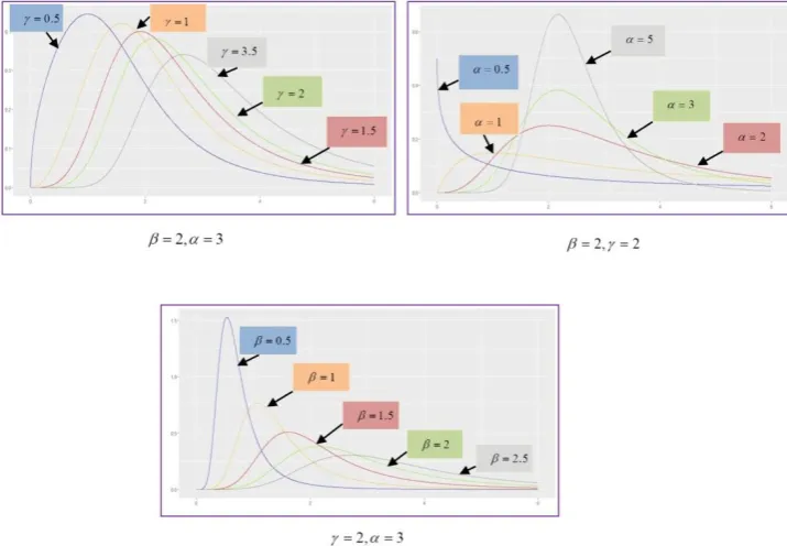
affects both tails. Figure 1 gives different shapes of the Kappa density function for various parameter specifications. The rth central moment of the Kappa distribution can be written as( / ) (1 / )
( )
( ) r
r r r
E X
,
where (.) denotes the gamma function. Furthermore, the variance, skewness and kurtosis are obtained as follows:
2 2 2
2
( ) ( 2 / ) (1 2 / ) ( 1 / ) (1 1 / )
( )
( )
Var X
2 3
3 2 1 1
3/2 2
2 1
( ) 3 ( ) 2 ( )
( )
Skewness X
,
3 2 2 4
4 3 1 2 1 1
2 2
2 1
( ) 4 ( ) 6 ( ) 3 ( )
( )
Kurtosis X
Where, i (
i/ ) (1
i/ );
i1, 2,3, 4. Moreover, the risk management has been intensively used in finance and insurance business. The value at risk is an important measure in risk management. Value at risk is defined as the worst expected loss over a given period at the specified confidence level (
). Mathematically,( )
P X VaR
, where X is the profit (loss) of the investment over the given time horizon. Also, the statistical loss distribution plays a key role in evaluating the value at risk measure. The main aim of this paper is to evaluate the VaR using the Kappa distribution. Based on the Equation (2), the VaR can be written as:ˆ ˆ
1 1/ 1/ ˆ
( ) ( ) ( 1)
VaR X F x
.Vol.4 / No.14 / Summer 2019
Figure 1. Different shapes of the Kappa density function for various parameter specifications
2. Literature Review
The value at risk is one of the oldest risk measures, which is basically defined as the maximum expected loss for a given probability. In the recent years, this measure has gained some attention among researchers and interesting results have been obtained. For example, Swami et al. (2016) estimated the value at risk for foreign exchange rate risk in India. They used the parametric variance-covariance and non-parametric historical simulation methods and showed that the t-students model can be considered as an adequate model for value at risk estimation. Dupuis et al. (2015) considered a new bias-robust conditional variance estimators based on weighted likelihood at heavy-tailed models for computing the value at risk measure. Mentel (2013) studied the parametric, nonparametric and semi-parametric models for estimating the value at risk. Results of this research indicate that the fat tail distributions present a good performance. Gebizlioglu et al. (2011) considered the Weibull distribution and its quantiles in the value at risk estimation. They used different estimation methods and showed that the maximum likelihood estimators have the best results for predicting the value at risk. Čorkalo (2011) compared the main approaches of calculating VaR and implements
distributional assumptions. Wong et al. (2016) provided extensive comparison of out-of-sample volatility and VaR forecast performance on different equity market indices using 13 risk models. Their results indicated that realized volatility models outperform GARCH models for volatility forecasts, but a simple EGARCH model outperforms the rest models for most of the VaR forecasts. Moreover, the heavy tailed distributions play an important role in value at risk estimation. The Kappa distribution is one of the heavy tailed distributions, which has useful properties. Due to its practicality, several authors have considered its properties, inferential methods and applications; for example, Kjeldsen et al. (2017) used the Kappa distribution in regional frequency analysis. Kim (2015) studied the Kappa distribution to analyze the effects of globalization by understanding differences and similarities among Asian countries and developed countries before and after the crisis. Jeong et al. (2014) proposed this distribution for hydrologic application. Livadiotis and McComas (2013) examined the physical foundations and theoretical development of the Kappa distribution. Kumphon (2012) studied the maximum entropy and maximum likelihood estimation methods for evaluating the parameters of the Kappa distribution. Pierrard and Lazar (2010) analyzed the various theories proposed for the Kappa distributions and their valuable applications in coronal and space plasmas. Ashour et al. (2009) and Dupuis and Winchester (2007) considered the different estimation methods for this distribution under complete and censored samples. Considering that so far any research has not used the Kappa distribution to evaluate the value at risk. Therefore, we want to present certain estimation methods for value at risk as a quantile of a Kappa distribution.
3. Methodology
3.1. Different Estimation Methods
Under classical paradigm, a number of estimation methods are available in statistical literature. But we shall be providing here only four of such methods, namely MLE, ME, PE and MPS.
3.1.1. Maximum Likelihood Estimator
This section deals with deriving MLEs of the unknown parameters of a Kappa( , , )
distribution. Suppose that X(X1,...,Xn) is a sample of size n from a( , , )
Kappa
distribution. Based on theobservation, the likelihood function can be given as follows:
1 ( 1)
1
( , , ) (1 ( / ) )
n
i i
i
L
x x
.(4)
Then, the log-likelihood function in (4) can be written:
1 1
( , , ) log( ( , , )) log log log
( 1) log ( 1) log(1 ( / ) )
n n
i i
i i
l L n n
x x
. (5)
Here, we assume that the parameters
,
and
are unknown. To obtain the normal equations for the unknown parameters, we differentiate (5) partially with respect to
,
and
and equate to zero as:1
1 ( , , )
log log
( / ) log( / )
( 1) 0
1 ( / )
n
i i
n
i i
i i
l n
n x
x x
x
1
1 ( , , )
( 1) 0
1 ( / )
n i
i i
x
l n
x
,And
1
1 ( , , )
log log
log(1 ( / ) ) 0
n
i i
n
i i
l n
n x
x
.
It is observed that the estimations cannot be obtained in closed forms. Numerical methods, such as the Newton-Raphson method, can be used here to solve the above non-linear equations.
3.1.2. Moment Estimators
Vol.4 / No.14 / Summer 2019
1
1 1
( ) (1 )
1 ( ) n i i x n
, 2 2 1 2 2( ) (1 )
1 ( ) n i i x n
, and 3 3 1 3 3( ) (1 )
1 ( ) n i i x n
.3.1.3. Percentile Estimators
Estimation based on percentiles was originally explored by Kao (1958). Let
X
1:n,...,
X
n n: be the order statistics of a random sample of size n from( , , )
Kappa
distribution. Ifp
idenotes anestimate of F x( i n: , , , )
, then the percentile estimators of the parameters
, and
can be obtained by minimizing, with respect to
, and
the function:
ˆ ˆ
1 1/ 1/
: :
1 1
ˆ
( ) ( 1)
n n
i n i i n i
i i
x F p x p
, (6)
with respect to
, and
. Here, piis taken as1
i
n , So based on the Kappa distribution the
Equation (6) can be rewritten as:
ˆ 1/ ˆ 1 1/ : : 1 1 ˆ
( ) ( ) 1
1
n n
i n i i n
i i
i
x F p x
n
.3.1.4. Maximum Product of Spacings
Cheng and Amin (1983) suggest a simple method for obtaining the estimation of the parameters of continuous distributions. Based on the Equation (1), the product spacings can be written as:
1 : 1: 1 1 : 1: 1 ( , , ) ( , , , ) ( , , , )
(1 ( / ) ) (1 ( / ) )
n
i n i n
i
n
i n i n
i
F x F x
x x
and the log likelihood is:
1 :
1
1:
(1 ( / ) )
log ( , , ) log
(1 ( / ) )
n i n
i i n x x
(7)The maximum product of spacing estimates of the unknown parameters can be obtained using the following non-linear equations:
1 1
: : :
: 1:
1
1
1: 1: 1:
: 1:
( / ) log( / )(1 ( / ) ) log ( , , )
(1 ( / ) ) (1 ( / ) ) ( / ) log( / )(1 ( / ) )
(1 ( / ) ) (1 ( / )
n
i n i n i n
i n i n
i
i n i n i n
i n i n
x x x
x x
x x x
x x
0, ) 1 1 1
: : : 1: 1 1 1 1: 1: : 1:
( ) (1 ( / ) ) log ( , , )
(1 ( / ) ) (1 ( / ) ) ( ) (1 ( / ) ) 0,
(1 ( / ) ) (1 ( / ) ) n
i n i n
i n i n
i
i n i n
i n i n
x x x x x x x x
And : : : 1: 1 1: 1: : 1:(1 ( / ) ) log(1 ( / ) ) log ( , , )
(1 ( / ) ) (1 ( / ) ) (1 ( / ) ) log(1 ( / ) ) 0.
(1 ( / ) ) (1 ( / ) )
n
i n i n
i n i n
i
i n i n
i n i n
x x x x x x x x
4. Results
Application in Insurance Stock Prices
considered in financial data. We obtained the different criteria as:
Akaike Information Criterion:
2
2ln
Akaike
. Bayesian Information Criterion:
ln( )
2ln
Bayesian
n
. Likelihood Criterion:
1
ln
ln(
( ))
ni i
Likelihood
f x
. Kolmogrov-Smirnov Distance:
( , ] 1
1
sup
;
n
n n x i
i
KS
F
F
F
I
X
n
. Anderson-Darling Distance:
2
( , ] 1
(
)
1
;
(1
)
n n
n x i
i
F
F
AD
n
dF
F
I
X
F
F
n
.Where,
( , ]
1;
0;
x
X x
I
otherwise
and
&
are the number of parameters and likelihood function respectively. The results for different distributions are: Kappa distribution:
100
1
100
7.466043 1
( ) 2(3) 2(100 log(7.466043) (100 7.466043 0.228924) log(5.158308)
log(0.228924) (7.466043 0.228924 1) log
(0.228924 1) log(1 ( / 5.158308) )) 384.6223,
i i
i i
Akaike Kappa
x
x
100
1
100
7.466043 1
( ) 13.8155 2(100 log(7.466043) (100 7.466043 0.228924) log(5.158308)
log(0.228924) (7.466043 0.228924 1) log
(0.228924 1) log(1 ( / 5.158308) )) 392.0378, i i
i i
Bayesian Kappa
x
x
100
1
100
7.466043 1
( ) 100 log(7.466043) (100 7.466043 0.228924) log(5.158308)
log(0.228924) (7.466043 0.228924 1) log
(0.228924 1) log(1 ( / 5.158308) )) -189.3111,
i i
i i
Likelihood Kappa
x
x
( )=0.1130957
KS Kappa and
AD Kappa
(
) 2.0302055
Gamma distribution:
3.380695
100100
( /1.037421) 3.380695 1
1
( ) 4 2 log (1.037421) (3.380695)
xi 395.7132,
i i
Akaike Gamma
x e
3.380695
100100
( /1.037421) 3.380695 1
1
( ) 9.21 2 log (1.037421) (3.380695)
xi 400.9235,
i i
Bayesian Gamma
x e
3.380695
100100
( /1.037421) 3.380695 1
1
( ) log (1.037421) (3.380695)
xi -195.857,
i i
Likelihood Gamma
x e
( ) 0.169257
Vol.4 / No.14 / Summer 2019
Weibull distribution
2.216181
100
100
( /3.956465) 2.216181 1
1
( ) 4 2 log (2.216181/3.956465)
( / 3.956465) xi =386.8964,
i i
Akaike Weibull
x e
2.216181
100
100
( /3.956465) 2.216181 1
1
( ) 9.21 2 log (2.216181/3.956465)
( / 3.956465) xi =392.1068,
i i
Bayesian Weibull
x e
2.216181 100
100
( /3.956465) 2.216181 1
1
( ) (2.216181/3.956465)
( / 3.956465) xi -191.4482,
i i
Likelihood Weibull
x e
( ) 0.127438
KS Weibull and AD Weibull( )2.977904.
Burr distribution:
100 100 8.006705 1
1
100
8.006705 0.111670 1 1
( ) 4 2 log (0.111670 8.006705)
(1 ) 476.0898,
i i
i i
Akaike Burr x
x
100
100 8.006705 1
1
100
8.006705 0.111670 1
1
( ) 9.21 2 log (0.111670 8.006705)
(1 ) 481.3002,
i i
i i
Bayesian Burr x
x
100
100 8.006705 1
1
100
8.006705 0.111670 1
1
( ) log (0.111670 8.006705)
(1 ) 236.044,
i i
i i
Likelihood Burr x
x
( ) 0.328569
KS Burr and AD Burr( )13.13082.
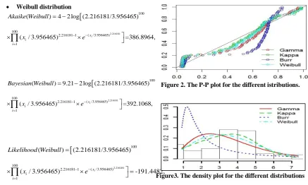
Figure 2. The P-P plot for the different istributions.
Figure3. The density plot for the different distributions
Based on different criteria, it is observed that the Kappa distribution has smallest Akaike, Bayesian, KS and AD values. Also, it has largest likelihood value, so, the Kappa distribution can be considered as an adequate model for analyzing the proposed data. Figures 2 and 3 show the P-P plot and the density plots for the four different proposed distributions. The figures show that the Kappa distribution provides the best fit. Now, we obtained the unknown parameters of the Kappa distribution using maximum likelihood, maximum product of spacing, moment and percentile methods. The results for different methods are given by:
Maximum Likelihood Estimator (MLE)
7.466043
,
5.158308
,0.228924
. Maximum Product of Spacings (MPS)
7.422851
,
5.136978
,0.208943
. Moment estimator (ME)
7.52634
,
6.06546
,0.237385
Percentile Estimator (PE)
7.44983
,
5.14997
,0.213265
.Based on the Hannan–Quinn information criterion (HQC), we compared the above estimators as:
100
1
100
7.466043 1
2(100 log(7.466043) 170.915642 log(5.158308) 100 log(0.228924) 0.7091564 log
(1.228924) log(1 ( / 5.158308) ) 6 log(log(100)) 387.78535,
i i ML
i i
E
H
x Q
x
100
1
100
7.422851 1
2(100 log(7.422851) 155.095275 log(5.136978) 100 log(0.208943) 0.5509527 log
(1.208943) log(1 ( / 5.136978) ) 6 log(log(100)) 388.8093,
SP
i M
i i
i
x
x HQ
100
1
100
7.52634 1
2(100 log(7.52634) 178.664022 log(6.06546) 100 log(0.237385) 0.7866402 log
(1.237385) log(1 ( / 6.06546) ) 6 log(log(100)) 402.9454,
i i ME
i i
H
x Q
x
And
100
1
100
7.44983 1
2(100 log(7.44983) 158.878799 log(5.14997) 100 log(0.213265) 0.5887879 log
(1.213265) log(1 ( / 5.14997) ) 6 log(log(100)) 388.339.
i PE
i i
i
x
x HQ
Now, we obtain the value at risk using the maximum likelihood, maximum product of spacing, moment and percentile methods as:
ˆ ˆ
1/ 1/
0.95
1/0.228924 1/7.466043
ˆ ( ) (0.95 1)
(0.95 1) (5.158308)=4.286811, VaR MLE
ˆ ˆ
1/ 1/ 0.95
1/0.208943 1/7.422851 ˆ ( ) (0.95 1) ( )
(0.95 1) (5.136978) 4.323762, VaR MPS
ˆ ˆ
1/ 1/
0.95
1/0.237385 1/7.52634
ˆ
( ) (0.95 1)
(0.95 1) (6.06546)=5.021131,
VaR ME
And
ˆ ˆ
1/ 1/
0.95
1/0.213265 1/7.44983
ˆ
( ) (0.95 1)
(0.95 1) (5.14997)=4.323997.
VaR PE
respectively. We finally compare the relative performances of the four estimators using the Hannan– Quinn information criterion. The maximum likelihood estimator gives the best performance. However, the percentiles and the maximum product of spacing estimators perform equally well and also the moment estimator gives the worst performance. For obtaining the VaR estimation, the different proposed estimators of the parameters have been inserted into the inverse cumulative distribution function of the Kappa loss function (
F
1( )
x
). It is observed that the results of the VaR estimation using the proposed methods are satisfactory.5. Discussion and Conclusions
Vol.4 / No.14 / Summer 2019
parameters. Based on different tests and criteria, it is observed that the Kappa distribution can be considered for modeling the data of the stock prices insurance well. We also observed that the value at risk is smallest using the maximum likelihood estimation method. The implication of our study is important and that is the value at risk can be evaluated using different estimation methods and based on the heavy tail distributions such as Kappa distribution, as adopted in the present work.
References
1) Abada, P., Benitob, S., Lópezc, C. (2014). A comprehensive review of Value at Risk methodologies. The Spanish Review of Financial Economics, 12, 1-46.
2) Ashour, S.K., Elsherpieny, E.A., Abdelall, Y.Y. (2009). Parameter Estimation for Three-Parameter Kappa Distribution under Type II Censored Samples. Journal of Applied Sciences Research, 5(10), 1762-1766.
3) Basu, B., Tiwari, D., Kundu, D., Prasad, R. (2009). Is Weibull distribution the most appropriate statistical strength distribution for brittle materials?. Ceramics International, 35, 237-246.
4) Brandolin, D., Colucci, S. (2012). Backtesting value-at-risk: a comparison between filtered bootstrap and historical simulation. Journal of Risk Model Validation, 13, 3-16.
5) Braione M., Scholtes, N.K. (2016). Forecasting Value-at-Risk under different distributional assumptions. Econometrics, 4, 1-27.
6) Cheng, R. C. H., Amin, N. A. K. (1983). Estimating parameters in continuous univariate distributions with a shifted origin. Journal of the Royal Statistical Society Series B (Methodological), 45, 394-403.
7) Čorkalo, S. (2011). comparison of value at risk approaches on a stock portfolio. Croatian Operational Research Review (CRORR), 2, 81-90.
8) Dupuis, D.J., Winchester, C. (2007). More on the four-parameter Kappa distribution. Journal of Statistical Computation and Simulation, 71, 99-113.
9) Dupuis, D.J., Papageorgiou, N., Rémillard, B. (2015). Robust Conditional Variance and Value-at-Risk Estimation. Journal of Financial Econometrics, 13:896–921.
10)
11) Gebizlioglu, O.L., Şenoğlu, B., MertKantar, Y. (2011). Comparison of certain value-at-risk estimation methods for the two-parameter Weibull loss distribution. Journal of
Computational and Applied Mathematics, 11, 3304-3314.
12) Hang, A. (2009). Value at risk estimation by quantile regression and kernel estimator. Review of Quantitative Finance and Accounting, 19(5),379-395.
13) Jeng, B.Y., Murshed, Md.S., Seo, Y.A., Park, J.S. (2014). A three-parameter Kappa distribution with hydrologic application: a generalized Gumbel distribution. Stochastic Environmental Research and Risk Assessment, 28, 2063–2074. 14) Johnson, B.A., Long, Q., Huang, Y., Chansky, K.,
Redman, M. (2016). Model selection and inference for censored lifetime medical expenditures. Biometrics, 72(3),731-41.
15) Kao, J.H.K. (1958). Computer methods for estimating Weibull parameters in reliability studies. IRE Transactions on Reliability and Quality Control, 13,15–22.
16) Kim, J. (2015). Heavy Tails in Foreign Exchange Markets: Evidence from Asian Countries. Journal of Finance and Economics, 3, 1-14.
17) Kjeldsen, T.R., Ahn, H., Prosdocimi, L. (2017). On the use of a four-parameter Kappa distribution in regional frequency analysis. Hydrological Sciences Journal, 62, 1354-1363.
18) Kumphon, B. (2012). Maximum Entropy and Maximum Likelihood Estimation for the Three-Parameter Kappa Distribution. Open Journal of Statistics, 2,415-419.
19) Livadiotis, G., McComas, D.J. (2013). Understanding Kappa Distributions: A Toolbox for Space Science and Astrophysics. Space Science Reviews, 175, 183–214.
20) Mentel, G. (2013). Parametric or Non-Parametric Estimation of Value-At-Risk. International Journal of Business and Management, 8,103-112. 21) Nwobi, F.N., Ugomma, C.A. (2014). A
Comparison of Methods for the Estimation of Weibull Distribution Parameters. Metodološki zvezki, 11, 65-78.
22) Ouarda, T.B.M.J., Charron, C., Shin,J.Y., Marpu, P.R., Al-Mandoos, A.H., Al-Tamimi, M.H., Ghedira, H., Al Hosary, T.N. (2015). Probability distributions of wind speed in the UAE. Energy Conversion and Management, 93, 414-434.
23) Panahi, H. (2016). Model Selection Test for the Heavy-Tailed Distributions under Censored Samples with Application in Financial Data. International Journal of Financial Studies, 4,1-14. 24) Panahi, H. (2017). Estimation Methods for the
Data. Communications in Mathematics and Statistics, 5,159-174.
25) Pierrard, V., Lazar, M. (2010). Kappa Distributions: Theory and Applications in Space Plasmas. Solar Physics, 267, 153-174.
26) Singh, S., Maddala, G. (1976). A Function for the Size Distribution of Income. Econometrica, 44, 963-970.
27) Sinha, P., Agnihotri, S. (2015). Impact of non-normal return and market capitalization on estimation of VaR. Journal of Indian Business Research, 7, 222-242.
28) Swami, O.S., Pandey, S.K., Pancholy, P. (2016). Value-at-Risk Estimation of Foreign Exchange Rate Risk in India. Asia-Pacific Journal of Management Research and Innovation, 12(1),1– 10.