A new approach for solving fuzzy multi-objective quadratic programming of water resource allocation problem

Journal of Industrial Engineering and Management Studies

Vol. 6, No. 2, 2019, pp. 78-102 DOI: 10.22116/JIEMS.2019.92259

www.jiems.icms.ac.ir

A new approach for solving fuzzy multi-objective quadratic

programming of water resource allocation problem

Seyed Hadi Nasseri1, Abdollah Baghban1,*, Iraj Mahdavi2

Abstract

This paper describes an application of fuzzy multi-objective quadratic model with flexible constraints for optimal allocation of limited available water resources among different water-user sectors. Due to the fact that, water resource allocation problem is one of the practical and essential subjects in real world and many of the parameters may be faced by uncertainty. In this paper, we present α - cut approach for transforming fuzzy multi-objective quadratic programming model with flexible constraints into a crisp form. By using this approach a multi-parametric multi-objective programming model corresponding to α and parameters of flexible constraints is obtained. One of the advantages of this model is that the α - cut level is not determined by the decision makers. Actually, this model itself can calculate the α - cut level. In order to achieve a desired Pareto optimal value of multi-parametric multi-objective model, we use goal programming method for illustration of water resource allocation with sensitivity analysis of lower bound of parameters in flexible constraints. To illustrate the efficiency of the proposed approach, we apply it for a real case problem of water resource allocation.

Keywords: Fuzzy multi-objective quadratic programming; Water resource allocation; Flexible constraints; α- cut approach; Sensitivity analysis.

Received: November 2018-20 Revised: February 2019-08 Accepted: February 2019-16

1. Introduction

Today, one of the most important issues for humans is access to fresh and clean water. As long as water demand is less than available, we are not facing the problem of allocating water resources. But with the growing population, development of industry and expansion of agriculture in arid and semi-arid areas, safe water supply has become one of the main challenges of the present century. Achieving a relative balance in the supply and use of water is a fundamental principle which is achieved through establishment of a comprehensive water management system. Therefore, scientists emphasize on the management of optimal water resources allocation (Archibald and Marshall, 2018). Actually, efficiently allocation of limited water resources is a critical problem for managers (Brown, Cochrane and Krom,

* Corresponding author; [email protected]

2010). Generally, maximizing the net economic benefit is a common objective for water resources allocation. However, water shortage has not been fully considered, thereby affecting the results of optimal water resource allocation. So, how to allocate optimal water from limited resources with the goal of increasing net economic benefit and reducing the water shortage is one of the most important problems that need to be solved (Wang, Zhang and Guo, 2018).

The development and application of mathematical science enable managers to formulate water resource allocation problems as mathematical optimization models. For example: Roozbahani et al. (Roozbahani, Schreider and Abbasi, 2013) modeled the problem of optimal water resource allocation to the agricultural sector in Sefidrood Basin in northern Iran as a linear programming model with net economic benefit objective. Babel et al. (Babel, Das Gupta and Nayak, 2005) modeled a bi-objective programming to optimal water resource allocation problem. In this model, two objectives are considered as maximizing the level of satisfaction and maximizing the net economic benefit. In solving this model, they used the weighted sum method to transform the multi-objective programming into single objective programming. Also, Rojanee Khummongkol et al. (Khummongkol, Sutivong and Kuntanakulwong, 2007) proposed an integrated multi-objective programming model for optimal water resource allocation to three main sectors: agricultural, domestic and industrial sector areas in the Rayong Province of Thailand. In this model, two objective functions are considered for maximizing net economic benefit and minimizing water shortage. They used a weighted sum method to solve his multi-objective programming model. Ijaz Ahmad et al. (Ijaz and Deshan, 2016) developed a deterministic water resource allocation model to optimally allocate limited available water resources among different water-use sectors. This model applied to the Hingol River basin in the Baluchistan Province of Pakistan. Two objective functions of the problem include maximizing the level of satisfaction and maximizing net economic benefit. They used of weighted sum method to solve multi-objective programming model.

In real world practical problems, since it's impossible to have access to complete and accurate information, uncertainty is considered as a very important factor in the water resource allocation. For example, Climate change, seasonal variations, water quality, demand, unexpected events, and so on (Archibald and Marshall, 2018). Hence, using uncertain parameters in these situations helps the associated manager to obtain more reasonable and realistic solutions. Hang Wang et al. (Wang, Zhang and Guo, 2018) developed an interval quadratic fuzzy dependent-chance programming model for optimal irrigation water allocation under uncertainty in the Minqin Oasis, the Wuwei city, northwest China with credibility level of the system revenue objective. Hamideh Hosseini Safa et al. (Hosseini Safa, Morid and Moghaddasi, 2012) presented a methodology that combine the uncertainty of both river flow forecasting and economic parameters for agricultural water allocation.

It is necessary to differentiate between flexibility in constraints and goal and uncertainty of the data. Flexibility is modeled by fuzzy sets and may reflect the fact that constraints or goal are

linguistically formulated. Their satisfaction is a matter of tolerance and degrees or fuzziness (Bellman and Zadeh, 1970). On the other hand, there is ambiguity corresponding to an objective variability in the model parameters (Randomness), or a lack of knowledge of the parameter values (epistemic uncertainty). Randomness originates from the random nature of events and it is about uncertainty regarding to the membership or non-membership of an element in a set. Epistemic uncertainty deals with ill-known parameters modeled by fuzzy intervals in the setting of possibility theory (Dubois, 1980; Zadeh, 1987). Also, Verdegay (Verdegay, 1982) proposed a parametric linear programming model with single parameter using α -cuts to achieve an equivalent model for the fuzzy linear programming with flexible constraints. Then he used duality results to solve the original fuzzy linear programming (Verdegay, 1984). Werner’s in (Werner’s, 1987) introduced an interactive multiple objective programming model subject to its constraint are flexible and proposed a special approach for solving multiple objective programming model basing on fuzzy sets theory. In the mentioned work, the classical model is extended by integration flexible constraints. After that, Delgado et al. (Delgado, Verdegay and Vila, 1989) a general model for fuzzy linear programming problem proposed. In particular, they suggested a resolution method for the mentioned problem. Campos et al. (Compose and Verdegay, 1989) considered a linear programming problem with fuzzy constraints including fuzzy coefficients in both matrix and right hand side. They dealt with an auxiliary model resulting from the embedding constraints in the main model. After that, Nasseri et al. (Nasseri and Ebrahimnejad, 2010) introduced an equivalent fuzzy linear model for the flexible linear programming problems and proposed a fuzzy primal Simplex algorithm to solve these problems.

In this paper, we present an approach based on α - cut for a fuzzy multi-objective quadratic programming model with flexible constraints. Using α - cut for each fuzzy parameters in objective functions, we transform these parameters into an interval number corresponding to

α. Then, fuzzy parameters are replaced with a convex linear combination of its corresponding interval. Also, each flexible constraint is replaced with a deterministic constraint, which some new parameters depend on. Furthermore, a multi-parametric multi-objective programming model is obtained. We propose goal programming method for solving this model. Finally, to illustrate the efficiency of the proposed method, we apply this method to the water resource allocation problem.

The main advantage of the proposed approach is flexibility in the obtained optimal solution so that it is associated to the minimum degree membership of the flexibility of the constraints. Also, the model is eligible to determine the optimal values of α - cut levels and convex linear combination coefficients in the fuzzy parameters of the objective functions, itself.

2. Preliminaries

In this section, we state some notions related to the considered problem. This following concept can be found in (Mansoori, Effati and Eshaghnezhad, 2018).

Definition 2.1 (Fuzzy set). Let X represents the universal set. Thus, the membership function of a fuzzy set Ais defined as _A:X [0,1].

To each member of x X , the membership function _A( )x attributes a real number in the range [0,1]and showing the membership degree of the member x in the set A. Each fuzzy set A with the membership function _A( )x can be shown as A 





x,_A

 

x



x X



. We show the set of all fuzzy numbers with E1.

Definition 2.2 (normal fuzzy set): The fuzzy set Ais normal if we have for at least one x X , _A

 

x 1.

Definition 2.3 (convex fuzzy set): A fuzzy set A is called convex if and only if for each

1, 2

x x X and 

 

0,1 , we have  _A



x₁ 



1 



x₂



min__A

 

x₁ ,_A

 

x₂ _.

Definition 2.4 (𝜶-cut set): For each [0,1], 𝛼 -cut set from a fuzzy set Ais defined as A_

with components x so that the values of the membership function _A( )x are not lower than

𝛼, which means A_ 



x _A

 

x 



.

Definition 2.5 (fuzzy number): A fuzzy number is a normal and convex fuzzy set whose membership function is continuous in fragmentation. Indeed, a fuzzy number A is a fuzzy set on the real numbers line, so that its membership function i.e. _A( )x , with conditions

1 2 3 4

a a a a

       has the following features:

 

 

1

1 2

2 3

3 4

4

0, , ( ) _1,

, 0,

L

A

R

x a

x a x a

x _{a x a}

x a x a

x a

 



  

   

 _{ }



 

  



(1)

Where, _L

 

x :_a a1, 2 _

 

0,1 is an increasing and continuous function and

 

3 4

 

: , 0,1

R x a a

 _  _ is a decreasing and continuous function.

Definition 2.6 (Trapezoidal Fuzzy Numbers): Each trapezoidal fuzzy number can be represented by quadruple A 



a a a a1, 2, 3, 4



_{so that its membership function is defined as}

1 1

1 2

2 1

2 3

4

3 4

4 3

4 0,

,

( ) 1, (2)

,

0,

A

x a

x a

a x a

a a

x a x a

a x

a x a

a a

x a

 

 

 _{ }

 _



  

 _

 _{ }

 

 _





The schema of a trapezoidal fuzzy number defined in (2) is shown in Figure 1.

Figure 1. The schema of a trapezoidal fuzzy number defined in the Definition 2.6

According to Definition 2.4, the 𝛼-cut set for a trapezoidal fuzzy number



1 2 3 4



, , ,

A  a a a a

can be shown with the following interval:

,

L U

A_  a a_{ } _ (3)

where,

 

1 1 2 1

L x a

a

a a



  

  _ 

 

  and

 

1 4

4 3

U a x

a

a a



  

  _ 

 

  . We note that by considering a2 a3,

the trapezoidal fuzzy number Awill change into a triangular fuzzy number; and if a1a2and

3 4

a a , to an interval number; and if a1 a2 a3a4, into a definite real number, which is a special case of a trapezoidal fuzzy number.

Definition 2.7 (arithmetic operations on 𝜶-cut sets): we assume that A_  a_L,a_U_ and

,

L U

B_  b_ b_ _are 𝛼-cut set of two fuzzy numbers AandB_{, respectively. The symmetry of}

the fuzzy number A is the fuzzy number A . Thus, if A_  a a_L, _U_ then

,

U L

A_  a_ a_

  _  _ and,

 









1. kA _min ka_L,ka_U , max ka_L,ka_U _,  k ,







2. AB _a_L b_L,a_U b_U_,







3. AB _a_L b_U,a_U b_L_,



 

   

4. AB ab _L, ab U_

   ,

Where,

 

ab _L min



a b_{ }U L,a b_{ }U U,a b_{ }L L,a b_{ }L U



and

 

ab U_ max



a b_{ }U L,a b_{ }U U,a b_{ }L L,a b_{ }L U



.

, ,

L U L U

a a b b

   

        if and only if aL bL,aU bU.

Definition 2.8 (flexible linear constraint): Consider a DM faced with a programming problem with linear constraints in which he /she can endure violation in completion at the constraints, that is he /she allow the constraints to be hold as well as possible. For each constraints in the constraints set, this assumption can be denoted by flexible linear constraint

F

i i

a x b and for eachi 1, 2,...,m modeled by use of a membership function:

 

 

1, , 0,

i i

i i i i i i

i i i

a x b μ x f x b a x b p

a x b p

 



_   

 _{ }



(4)

Where, f_i

 

. is strictly decreasing and continuous for a x_i , f_i

 

b_i 1 and f_i



b_i p_i



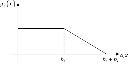
0. The figure of the membership function defined in (4)is shown in Figure 2.

Figure 2. The figure of the membership function defined in (4)

This membership function expresses that the DM tolerates violation in the accomplishment of the constraints i up the value b_i p_i. The function μ x_i

 

gives the degree of satisfaction of the i -th constrains for x  n.

3. Fuzzy multi-objective quadratic programming model with flexible

constraint

Consider a Fuzzy Multi-objective Quadratic Programming Model (FMOQPM) with flexible constraints as follow:

   

 

 

1 2

1

min , ,..., , , 1, 2,..., ,

. . , 1, 2,..., ,

0,

T T

K k k k

n

F ij j i j

F x F x F x F x x Q x C x k K

s t a x b i m

x



    

 







(5)

Where,



1, 2,...,



T n

x  x x x is a n-dimensional decision variable, each Qk    qijk _{n n} ,

1, 2,...,

k  K are fuzzy n n - dimensional positive definite hessian matrix in the k -th objective function and



1 2



, ,..., n

k k k k

C  c c c , k 1, 2,...,K are n- dimensional linear section of objective function with fuzzy components. Also, A    aij _{m n} is a real m n -dimensional

i

matrix of technical coefficients. The notation

 

F represents a fuzzy extension of

 

 on real line which is applied to compare the left side of fuzzy constraints with the right hand side (Nasseri and Ramzannia-Keshteli, 2018) .

In general, model (5) in not well-defined due to the following reasons: 1. The constraints

1

n

F

ij j i

j

a x b





, i 1, 2,...,m do not result in a deterministic feasible set. 2. Due to the existence of fuzzy values in each objective functionsF_k

 

x ,k 1, 2,...,K , there is no deterministic objective space.

If we want to define a deterministic feasible set, an idea is to provide confidence level β_i at which it is desired that the corresponding i -th fuzzy constraint hold. Therefore, in order to remove the first mentioned restriction, the following model can be introduced.

   

 

1 2

1

min , ,..., ,

. . , 1, 2,..., ,

0, , 0 1, 1, 2,...,

K

n

F

i ij j i i

j

D

i i i

F x F x F x

s t μ a x b β i m

x β β β i m

                 



(6)

To drive for a meaningful choice of membership function for each fuzzy constraint, it is disputed that if

1

n

ij j i j

a x b







, then i -th constraint is fully satisfied. If

1

n

i j j i i

j

a x b p



 



,

where p_i is the predefined maximum tolerance from zero as determined by the DM, then the i -th constraint is perfectly violated. For





1

,

n

ij j i i i

j

a x b b p



 



, the membership function is

monotonically decreasing. If this decrease is along with a linear function then it is sensible to select the membership function of the i -th constraint as:

 

1,

, 0,

i i

i i i

i i i i i

i

i i i

a x b b p a x

μ x b a x b p

p

a x b p

   _{ }  _      _{ }  (7)

We rewrite the model (6) as follows:

   

 





1 2

min , ,..., ,

. . 1 , 1, 2,..., ,

0, , 0 1, 1, 2,...,

K

i i i i

D

i i i

F x F x F x

s t a x b p β i m

x β β β i m

 

 

   

    

(8)

Now, we are going to give the concept of feasible solution to the fuzzy multi-objective quadratic programming model in form (8).

Definition 3.1. Let β 



β β₁, ₂,...,β_m





 

0,1mbe a vector, and







n| 0, 1 , D, 1, 2,...,



β i i i i i i

A vector x X_βis called β - feasible solution to the model (8).

Following proposition allows us to define the feasible set for the model (8) as an intersection of all β -cutcorresponding to flexible constraints.

Proposition 3.1. Let β 



β β₁, ₂,...,β_m





 

0,1m then

1

i

m i

β β

i

X X



 , where







| 0, 1 ,



i

i n D

β i i i i i i

X  x  x  a x  b p β β β (10) For i 1, 2,...,m. Actually,

i

i β

X is the β_i -cut of the i -th fuzzy constraint.

Proof. For any



1, 2,...,



 

0,1

m m

β  β β β  , let x X_β , therefor β_i β_iDand



1



i i i i

a x  b p β . Now from (10), we have

i

i β

x X ,i 1, 2,...,m.Therefor,

1

i

m i β i

x X



 .

On the other hand, if

1

i

m i β i

x X



 , we have

i

i β

x X for all i 1, 2,...,m.Therefor,



1



i i i i

a x  b p β ,β_i β_iD and x 0. Hence, x X_β .

Proposition 3.2. Let β



β β₁ , ₂,...,β_m



and β



β β₁ , ₂,...,β_m



, where β_iβ_i for all

1, 2,...,

i  m then β-feasibility of x implies the β-feasibility of it.

Proof. Let x X _β is a β- feasible solution of the model (8). We have x 0,



1



i i i i

a x  b p β and β_i β_iD for i 1, 2,...,m. from β_iβ_i, we have



1



i i i i

a x  b p β and β_i β_iD. So, x X_β.

Remark 3.1. If the model (6) is not infeasible then X_β is not empty. Proof. For a given β 

 

0,1 , let n

x  be a β - feasible solution to (8) (a solution with the same degrees of satisfaction in all of constraints). This means that x satisfy the equations



1



i i i i

a x  b p β , 0β_i 1, β_i β_iDand x 0 or equivalently, x X_β.

3.1. Proposed approach

In order to overcome the second mentioned restriction in model (5), we present a new approach based on the definition of α - cut for a fuzzy number. Definition 3.2 (Panigrahi, Panda and Nanda, 2008). Suppose F:  n E1is a fuzzy function where  is an open subset of n. The 𝛼-cut set F at u is shown as

 

( , ) ,L



,



U

F u _  f u  f u  _ that is a closed and bounded interval. Here, f u( , ) L and ( , )U

Theorem 3.1. A fuzzy function F C: E1 defined on a convex subset C in  is convex, if and only if, F





1



x y



 



1 

  

F x F y

 

for every x and y in C and

 

0,1 . A fuzzy function F C: E1 defined on a convex subset C in  is called strictly convex if







1





1

  

 

F  x y   F x F y for each 

 

0,1 and for every x and y in C such that x y (Wang and Wu, 2003).

Theorem 3.2. Suppose that C is a convex subset in  and 1 :

F C E is a fuzzy function then F is convex if and only if for each given 

 

0,1 ,



f

 

x



_Land



f

 

x



U_ are convex functions in x (Wang and Wu, 2003).

Proof. See (Wang and Wu, 2003). 

Using the concept of the  -cut in Definition 2.4, Definition 2.6 and Definition 3.2, for each fuzzy objective function in the model (5), we have:

 



_k



L,



_k

 



U T

   

_{k α}L, _{k α}U T

   

_{k α}L, _k U_α , 1, 2,...,

α α

f x f x x q q x x c c k K

 _   _   _

   

 

(11)

Where,

 

_k L_α

 

_ijk L

α _{n n}

q q     _ _ ,

 

 

U U k

k _α ij _α

n n

q q



 

 _ _ ,

 

 

₁

L

L i

k _α k _α

n

c c



 

 _ _ ,

 

 

₁

U

U i

k _α k _α

n c c     _ _ and,

 





 

 

 





 

 

, 1, 2,..., , 1, 2,...,

L T L T L

k _α k _α k _α

U _T U _T U

k _α k _α k _α

f x x q x x c k K

f x x q x x c k K

  

   (12)

In equations (12), the values of



_k

 



L

α

f x and



_k

 



U

α

f x are called the optimistic and pessimistic values for each objective function F_k

 

x , respectively.

Remark 3.2. In the objective function of the maximizing type, conversely minimization type, the values of



fk

 

x



_αL and



 



U

k _α

f x are called the pessimistic and optimistic values for each objective function F_k

 

x , respectively.

By placing equations (11) and (12) in the model (8), we have:

 







 





 





 





 





 







1 1 2 2

min , , , ,..., , ,

. . 1 , 1, 2,..., ,

0, , 0 1, 1, 2,...,

L U L U L U

K K

α α α α α α

i i i i

D

i i i

f x f x f x f x f x f x

s t a x b p β i m

x β β β i m

                       (13)

We consider a convex linear combination from



f_k( )x



_L and



f_k( )x



U_ for each

1, 2,...,



 













 





  









1 1 2 2

min , , , , , ,..., , , ,

. . , , 1 , 1, 2,..., ,

1 , 1, 2,..., ,

0, , 0 1, 1, 2,..., ,

0 1, 1, 2,..., .

K K

L U

k k k k _α k k _α

i i i i

D

i i i

k

f x α t f x α t f x α t

s t f x α t t f x t f x k K

a x b p β i m

x β β β i m

t k K

 

 

   

   

    

  

(14)

We identify the model (14) as Multi-Parametric Multi-objective Programming Model (MPMOPM).

Actually, determining the amount of  and linear combination coefficients will be responsibility of the model and will be considered as a decision variable in the model.

In the next, we are going to give the concept of efficient solution to the MPMOPM in form (14).

Proposition 3.3. If x X_ be a β - feasible solution to the model (5), then there are at least one 

 

0,1 and t

 

0,1K such that



x α t, ,



 n K 1is a β - feasible solution to the model (14) and



x α t, ,



X_β.

Proof. It is clear. 

Definition 3.3.The β - feasible solution



x α t, ,



 n 

 

0,1K1 is called a weakly efficient solution for the model (14) if there is no β- feasible solution



x α tˆ, ,ˆ ˆ



 n

 

0,1K1, so that for each k 1, 2,...,K _, f_k



x α tˆ, ,ˆ ˆ_k



f_k



x α t, , _k



. Additionally, if there is no



_ˆ



 

1

ˆ

ˆ, , n 0,1K

x α t    , so that for each k 1, 2,...,K , f_k



x α tˆ, ,ˆ ˆ_k



f_k



x α t, , _k



, then



x α t, ,



is called an efficient solution to the model (14).

Pay attention that any efficient solution to the model (14) is an efficient solution to the model (5). In the following theorem, we represent the necessary and sufficient condition for an efficient solution to the model (5).

Theorem 3.3. Let



1, 2,...,



 

0,1

m T

m

β  β β β  , and x X_ be a β - feasible solution to the model (5). Then, x is an efficient solution to the model (5), if and only if there is at least one

 

0,1 

 and t 

 

0,1Ksuch that



x α t, ,



be an efficient solution to the model (14).

Proof. Assume that x X_ is an efficient solution to the model (5), then for all xˆX_ concludes that F_k

 

x F_k

 

xˆ for any k 1, 2,...,K . According to equation (12), for any

 

ˆ

,  0,1

  and k 1, 2,...,K , F_k

 

x  



f_k

 

x



_αL,



f_k

 

x



U_α _

  and

 

ˆ



 

ˆ



L_ˆ,



 

ˆ



U_ˆ

k k _α k _α

F x   f x f x _

 . So,



 



,



 





 

ˆ



ˆ,



 

ˆ



ˆ

L U L U

k _α k _α k _α k _α

f x f x f x f x

  _ 

   

   

 





L



₁





 



U ˆ



 

_ˆ



L_ˆ



₁ ˆ





 

_ˆ



U_ˆ

k _α k _α k _α k _α

t f x  t f x t f x  t f x

Then f_k



x α t, ,



f_k



x α tˆ, ,ˆ ˆ



for all k 1, 2,...,K . That's mean



x α t, ,



is an efficient solution to the model (14).

On the contrary, assume that



x α t, ,



is an efficient solution to the model (14). According to Definition 3.3, for each k 1, 2,...,K and



x α tˆ, ,ˆ ˆ



X_β, we _have:



_{ˆ, ,ˆ} ˆ





_{, ,}



k k k k

f x α t f x α t . Then,

 





L



1





 



U ˆ



 

ˆ



L_ˆ



1 ˆ





 

ˆ



U_ˆ

k _α k _α k _α k _α

t f x  t f x t f x  t f x

Since, according to equation (12), for all k 1, 2,...,K , _k

 



_k

 



L,



_k

 



U

α α

F x   f x f x _

 

and _k

 

ˆ



_k

 

ˆ



L_ˆ,



_k

 

ˆ



U_ˆ

α α

F x   f x f x _

 , hence Fk

 

x Fk

 

xˆ . That's mean x is an efficient

solution to the model (5). 

In Theorem 3.3, we have provided a computational method to solve multi-objective quadratic programming with flexible linear constraint (5). Thus by assigning a specific β by DM, we may replace the β_i in the corresponding constraint of (14), and solve the resulted model to compute the efficient solution to the model (14). An efficient solution to (14) has three characteristics:

1. The solution has various satisfaction degrees corresponding to each constraint. 2. The acquired solution is efficient solution to the model (5).

3. The amount of α for computing α -cut of fuzzy values in the model is obtained by solving model, without judgment of the DMs.

This solution permits DM to obtain a more flexible and more compatibility by assigning desired preferences, especially, in online optimization in more noticeable.

Actually, In Theorem 3.3, a method for solving fuzzy multi-objective quadratic programming model with flexible linear constraints is introduced for obtaining an efficient solution.

Now, we are going to introduce our algorithm steps for solving a fuzzy multi-objective quadratic programming with flexible linear constraint.

Algorithm I. (Algorithm steps for solving a model in form (5)) Step1. _The β_iD- level to each β_i is determined by the DM.

Step2. Obtain the corresponding α -cut interval based on equation (3) for each fuzzy value in the model.

Step3. Create the corresponding MPMOPM similar to the model (14).

In the next section, we introduce a classical method for obtaining an efficient solution to the model (14).

3.2 Goal programming method for solving MPMOPM

This method is used to solve multi-objective decision making problems to find efficient solutions. Generally, a multi-objective programming model can be shown as follows:

   

 

1 , 2 ,...,

. .

k

Min F x F x F x

s t x X

 

 

 (15)

where, F_k

 

x is k -th objective function of this model and X represents the feasible set. Goal programming is an one of the most powerful multi-objective technique which is based on the distance function where the DM looks for the solution that minimize the absolute deviation between the achievement level of the objective and its aspiration level. It can be stated in the following program (Charnes and Cooper, 1959):

 

1

. .

K

aspiration

k k

i

Min F x f

s t x X









₍₁₆₎

where, f_kaspiration is the aspiration level of the k - th objective F_k

 

x for any k 1, 2,...,K . In goal programming method, the distance between F_k

 

x and f_kaspiration, that's mean

( ) aspiration

k k

F x f , is expressed by the deviational variable y_k and y_k for any

1, 2,...,

k  K , where y_k is the positive deviational variable,

 





max 0, aspiration

k k k

y  F x f and y_k is the negative deviational variable,

 





max 0, aspiration

k k k

y  f F x . When our objective function is a maximization type, we want F_k

 

x f_kaspiration, so, minimize the y_k. Also, when our objective is a minimization type, we want F_k

 

x f_kaspiration, so, minimize the y_k. Furthermore, when we want to have

 

aspiration

k k

F x f , we need to minimize y_ky_k. In this case, the goal programming model according to model (15) is as follows:

 

1

. . , 1, 2,..., ,

0, 0, 1, 2,..., ,

K

k k

i

aspiration

k k k k

k k

Min y y

s t F x y y f k K

x X

y y k K

 



 

 



   



  



(17)

One of the challenges of the goal programming method is to choice the aspiration level to each objective function. There are several ways to choice the aspiration level, for example, by DMs or can be equal to the ideal value of each objective function which, we define in the next.

Definition 3.3. (Ideal value): The value of f_kI is the ideal value of F_k

 

x in model (15) and is calculated as follows (Ehrgott and Wiecek, 2005):

 

min . .

I

k k

f F x

s t x X



 (18)

By solving the single objective model (18) for any k 1, 2,...,K , the ideal values f_kI are obtained.

Theorem 3.4. Every optimal solution to the model (16) is an efficient solution to the model (15) (Gandibleux, 2002).

By using goal programming method for solving MPMOPM (10), we have:











 





  









1 min

. . , , , 1, 2,..., ,

, , 1 , 1, 2,..., ,

1 , 1, 2,..., ,

0, , 0 1, 1, 2,..., ,

0 1, 1, 2,..., ,

0, 0, 1, 2,..., .

K

k k

k

aspiration

k k k k k

L U

k k k k _α k k _α

i i i i

D

i i i

k

k k

y y

s t f x α t y y f k K

f x α t t f x t f x k K

a x b p β i m

x β β β i m

t k K

y y k K

 



 

 



   

   

   

    

  

  



(19)

We identify the model (19) as Multi Parametric Goal Programming Model (MPGPM). Remark 3.4. In the MPGPM, we consider the value of f_kaspirationequal to the ideal value f_kI . In the following algorithm, we summarize presented method to solve the fuzzy multi-objective quadratic programming with flexible constraints.

Algorithm II (proposed algorithm)

Step1. We use the Algorithm I to achieve the MPMOPM.

Step2. Solve the model (18) corresponding to MPMOPM for obtaining the ideal value of each objective function.

Step3. _{Solve the MPGPM corresponding to MPMOPM. Then, obtain the optimal solutions}

x , α , t , β and the optimal value of each objective function f_k



x α t, ,



, for every 1, 2,...,

Step4. If the DMs accept the optimal value of each objective function, STOP. Else, go to Step1 and change the value of β_iD- level to each β_i .

4. Water resource allocation problem

In this section, we present a multi-objective quadratic programming model with flexible constraint to water resource allocation problem. This model is an extension of the presented model by (Babel, Das Gupta and Nayak, 2005). The presented model by them is modeled in certain environment. We extend this model to uncertainty environment. Also, we consider the flexible constraints for this model.

Assume that the water resource problem is to find the amount of water allocation to each three sector; domestic, industrial and agriculture from one resource. For this propose, two objective

functions are considered: the first objective is to minimize shortage and the second objective is to maximize the net economic return.

In order to minimize the amount of shortage and maintain justice, we consider the first objective function as follows:





 

2

1 2

1 min

n

i i

i

i

d x

F

d 







(20)

Where nis the number of irrigation area, x_i is decision variable and represents the allocated water for area i(1000m3)and d_iis the demand of water in area i(1000m3).

The allocation of water should be in such a way as to have economic justification. The second objective function models net economic returns and it is represented as follow;



1



2

max max

n

i i

i

x NER

F

Q R NER



 

 



(21)

where NER_iis the net economic return per one unit of water in area



3



$ 1000

i US m , Q is

the amount of water in resource



3



1000m and R is the amount of water that must remain in the resource



1000m3



so,



Q R



is available water



1000m3



, and NER_max is the maximum net economic return among considered areas



US$ 1000m3



.

The 2n1constraints are considered to this problem as follows:





1

n F i i

x Q R







(22)

, 1, 2,...,

F

i i

x d  i n (23)

0, 1, 2,...,

i

The constraint expressed in (22) models the amount of available water which is considered as a flexible constraint. The constraints (23) show the maximum water supply. These constraints are considered as flexible constraint too. The constraint (24) shows the non-negative constraint for allocated water.

This problem is formulated as fuzzy bi-objective quadratic programming model with



n1



flexible constraints. We solve this model with the proposed algorithm and the results are presented in the next section.

5. Numerical results

The example is built on the available data and information is for the Nong Pla Lai Reservoir in Chonburi Province in Eastern Thailand (Babel, Das Gupta and Nayak, 2005). In this paper, we

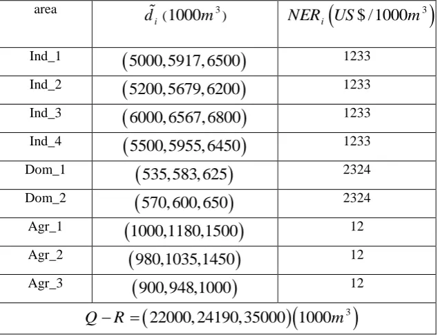
consider some of the crisp values as fuzzy values, such as demand and available water. The required inputs for application in the optimization process are provided in Table 1.

Table 1. Required inputs for water resource allocation

area

i

d (1000m3) NER USi



$ /1000m3



Ind_1



_{5000,5917, 6500}



1233 Ind_2



_{5200,5679, 6200}



1233 Ind_3



_{6000, 6567, 6800}



1233 Ind_4



_{5500,5955, 6450}



1233 Dom_1



_{535,583, 625}



2324 Dom_2



_{570, 600, 650}



2324 Agr_1



_{1000,1180,1500}



12 Agr_2



_{980,1035,1450}



12 Agr_3



_900,948,1000



12 Q R



22000, 24190,35000 1000





m3



Now, we are going to obtain the optimal solution of the water resource allocation which is given in equations (20)-(24). The steps of the algorithm II are given in details.

Step1. The βiD- level for i 1, 2,...,n1 are determined by the DM as shown in Table 2. Table 2. The value of D

i

β for each flexible constraint

1

D

β 2

D

β 3

D

β 4

D

β 5

D

β 6

D

β 7

D

β 8

D

β 9

D

β 10

D

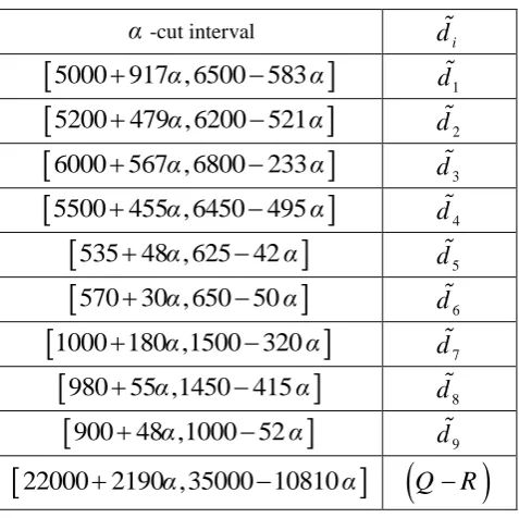
Step2. Obtain the corresponding α -cut interval based on equation (3) for each fuzzy number in this model as shown in Table 3.

Table 3. The α-cut interval for each fuzzy values

α -cut interval _di



5000 917 , 6500 583 α  α



d₁



5200 479 , 6200 521 α  α



d₂



6000 567 , 6800 233 α  α



d₃



5500 455 , 6450 495 α  α



d₄



535 48 , 625 42 α  α



d₅



570 30 , 650 50 α  α



d₆



1000 180 ,1500 320 α  α



d₇



980 55 ,1450 415 α  α



d₈



900 48 ,1000 52 α  α



d₉



22000 2190 ,35000 10810 α  α





Q R



Step3. Obtain the corresponding MPMOPM for water resource allocation problem as follows:

 



    



    





 

    





      

      

2 9

1 2

1

9

1 2

10 10 max

10 10 10 10

1

1 min , ,

1

max , ,

1

. . 1 1 , 1, 2,...,9,

1 1 ,

L U i i α i i α i

L U i

i i α i i α i i i

L U

α α

L U

i i i α i i α i i n

L U

i α α

i

t d t d x

f x α t

t d t d

x NER f x α t

t Q R t Q R NER

s t x t d t d β p i

x t Q R t Q R β p







  



 

 

    

      

       







(25)

10 10

0, D 1, D 1, 0 1, 0 1, 1, 2,...,9.

i i i i

x  β β  β β   t  α i 

The values of p_i are selected by the DMs. In this model, the selected values of p_i are shown in Table 4.

Table 4. The value of p_i for each flexible constraint

1

p p₂ p₃ p₄ p₅ p₆ p₇ p₈ p₉ p₁₀

Step4. Obtain the ideal value of each objective function. The ideal value of each objective function for water resource allocation model is



₁I, ₂I





0,1.0682



f f  .

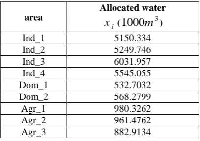
Step5. We solve the MPGPM corresponding to MPMOPM (25). Table 5 illustrate the allocated water to industrial areas (Ind_i), domestic areas (Dom_i) and agriculture areas (Agr_i) from solving the MPGPM using algorithm II by LINGO 17.0 software.

Table 5. The allocated water to each area from solving MPGPM using algorithm II

area

Allocated water

i

x (1000m3)

Ind_1 5150.334 Ind_2 5249.746 Ind_3 6031.957 Ind_4 5545.055 Dom_1 532.7032 Dom_2 568.2799

Agr_1 980.3262 Agr_2 961.4762 Agr_3 882.9134

The Pareto optimal values obtained for each objective function are



f f₁, ₂

 

 0.0011, 0.9250



.

One of the important parameters that affects the Pareto optimal value is the value of β_iD . In the next subsection, we are going to analyze the sensitivity of this model to the β_iD.

5.1 Sensitivity Analysis

We solved a multi-objective quadratic programming model with flexible constraints for water resource allocation problem using algorithm II. Now, we are going to evaluate sensitivity analysis for the Pareto optimal value by changing of some known parameters in Right-Hand-Sides such as β_i. Actually, the value of β_i determines the amount of deviation from demand and available water resource. According to model (25), when the value of β_i is closer to one, the amount of deviation from demand and available water resource decreases. That is, the DMs always want to bring the value of β_ito one.

In the following, we examine the sensitivity of the Pareto optimal values to variations of β_iD.

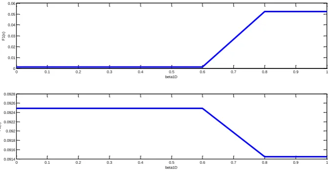
5.1.1 The sensitivity analyze for β₁D

As seen in Figure 3, the Pareto optimal value of f₁and f₂ for β₁Dfrom 0.0 to 0.6 are fixed and in their best values. By increasing the value of β₁D from 0.6 to 0.8, the Pareto optimal values f₁and f₂ to become worse. Also, for β₁Dfrom 0.8 to 1.0 the Pareto optimal values are fixed and in their worst values. So, the best value for β₁Dis in interval



0.0, 0.6 . Since, the



DMs want to close the value of β₁D to one, the best value for β₁Dis 0.6.

Figure 3. The sensitivity chart of each objective function based on changing β₁D from 0.0 to 1.0 5.1.2 The sensitivity analyze for β₂D

We change the value of β₂D from 0.0 to 1.0 as β₂D 0.0, 0.2, 0.4, 0.6, 0.8,1.0and solve the model (25). The obtained results of Pareto optimal value for each objective are shown in Figure 4. Corresponding to Figure 4, the results are similar to subsection 5.1.1. So, the best value for β₂Dis 0.6.

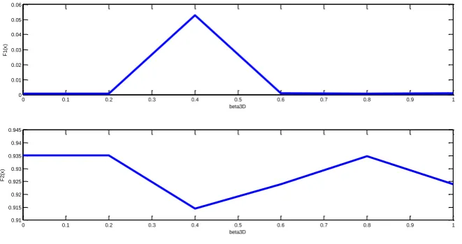
5.1.3 The sensitivity analyze for β₃D

Now, we examine the effect of β₃Don Pareto optimal value in the model (25). To do this, we consider β₃D 0.0, 0.2, 0.4, 0.6, 0.8,1.0and solve the model (25). The variations of Pareto optimal values for changing β₃D from 0.0 to 1.0 are shown in Figure 5. As shown in Figure 5, the Pareto optimal value of f₁ are fixed in



0.0, 0.2 and





0.6,1.0 . Also, by increasing the



value of β₃D from 0.2 to 0.4, the value of Pareto optimal of first objective function increases and gets worse. When β₃D rises from 0.4 to 0.6, the value of f₁ is reduced again. So, the best value of β₃D for first objective function is in



0.0, 0.2 and





0.6,1.0 .



0 0.1 0.2 0.3 0.4 0.5 0.6 0.7 0.8 0.9 1

0 0.01 0.02 0.03 0.04 0.05 0.06

beta1D

F

1

(x

)

0 0.1 0.2 0.3 0.4 0.5 0.6 0.7 0.8 0.9 1

0.0914 0.0916 0.0918 0.092 0.0922 0.0924 0.0926 0.0928

beta1D

F

2

(x

Given that the second objective function is maximization, the best value of β₃Dfor second objective function is in



0.0, 0.2 and 0.8. By intersection of the best value of



β₃D for f₁ and

2

f , the best and largest value for β₃Dis 0.8.

Figure 4. The sensitivity chart of each objective function based on changing β₂D from 0.0 to 1.0

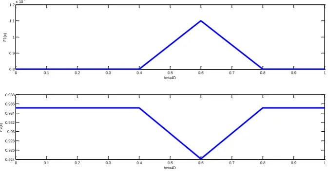
Figure 5. The sensitivity chart of each objective function based on changing β₃D from 0.0 to 1.0 5.1.4 The sensitivity analyze for β₄D

We change the value of β₄D from 0.0 to 1.0 asβ₄D 0.0, 0.2, 0.4, 0.6, 0.8,1.0. Figure 6 shown that the values of f₁ and f₂ are fixed in



0.0, 0.4 and





0.8,1.0 that are the best values of



them. Also, these functions get the worst their values for β₄D 0.6. According to Figure 6, the best value for β₄Dis 1.0.

0 0.1 0.2 0.3 0.4 0.5 0.6 0.7 0.8 0.9 1

0 0.01 0.02 0.03 0.04 0.05 0.06

beta2D

F

1

(x

)

0 0.1 0.2 0.3 0.4 0.5 0.6 0.7 0.8 0.9 1

0.0914 0.0916 0.0918 0.092 0.0922 0.0924 0.0926 0.0928

beta2D

F

2

(x

)

0 0.1 0.2 0.3 0.4 0.5 0.6 0.7 0.8 0.9 1

0 0.01 0.02 0.03 0.04 0.05 0.06

beta3D

F

1

(x

)

0 0.1 0.2 0.3 0.4 0.5 0.6 0.7 0.8 0.9 1

0.91 0.915 0.92 0.925 0.93 0.935 0.94 0.945

beta3D

F

2

(x

5.1.5 The sensitivity analyze for β₅D

By changing the value of β₅Dfrom 0.0 to 1.0 and solving the model (25), we obtain the results which are shown in Figure 7. By looking to Figure 6 and Figure 7, we observe that the obtained results are adverse. The best value for β₅D is 0.6 which is the worst value for β₄D.

Figure 6. The sensitivity chart of each objective function based on changing β₄Dfrom 0.0 to 1.0

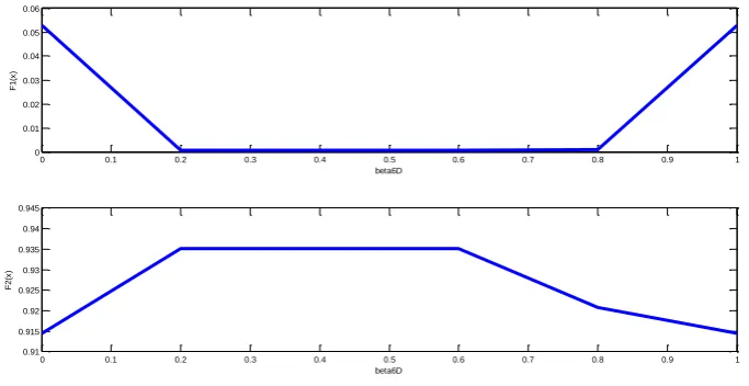
Figure 7. The sensitivity chart of each objective function based on changing β₅D from 0.0 to 1.0 5.1.6 The sensitivity analyze for β₆D

To show the effect of the value of β₆Don the Pareto optimal values of f₁ and f₂, we change the value of β₆D from 0.0 to 1.0. The changes in objective functions f₁ and f₂ are shown in Figure 8. When β₆Dis in interval



0.2, 0.7 , the first objective has the best value respect to



0 0.1 0.2 0.3 0.4 0.5 0.6 0.7 0.8 0.9 1

0.8 0.9 1 1.1 1.2x 10

-3

beta4D

F

1

(x

)

0 0.1 0.2 0.3 0.4 0.5 0.6 0.7 0.8 0.9 1

0.924 0.926 0.928 0.93 0.932 0.934 0.936 0.938

beta4D

F

2

(x

)

0 0.1 0.2 0.3 0.4 0.5 0.6 0.7 0.8 0.9 1

0 0.01 0.02 0.03 0.04 0.05 0.06

beta5D

F

1

(x

)

0 0.1 0.2 0.3 0.4 0.5 0.6 0.7 0.8 0.9 1

0.914 0.916 0.918 0.92 0.922

beta5D

F

2

(x

other value of β₆D. Also, the best value of β₆D for the second objective is in interval



0.2, 0.6 . Hence, the best value for



β₆D is 0.6.

Figure 8. The sensitivity chart of each objective function based on changing β₆D from 0.0 to 1.0 5.1.7 The sensitivity analyze for β₇D , β₈Dand β₉D

By changing the value of β₇Dfrom 0.0 to 1.0, we did not see any changes in the Pareto optimal value of objective functions. This result satisfy for β₈Dandβ₉D, too. In fact, the values ofβ₇D , β₈D and β₉D have no effect on the Pareto optimal value. Since the DMs are willing to increasing the value of β_i, we consider β₇D β₈D β₉D 1.

5.1.8 The sensitivity analyze for β₁₀D

The process of changing the values of f₁ and f₂ for different value of β₁₀D from 0.0 to 1.0 is shown in Figure 9. When β₁₀Drises from 0.0 to 0.8, the value of f₁ increases, unlike the value of f₂ . Also, when β₁₀D rises from 0.8 to 1.0, the values of f₁ and f₂decrease and increase, respectively and the desired value for β₁₀Dis zero.

0 0.1 0.2 0.3 0.4 0.5 0.6 0.7 0.8 0.9 1

0 0.01 0.02 0.03 0.04 0.05 0.06

beta6D

F

1

(x

)

0 0.1 0.2 0.3 0.4 0.5 0.6 0.7 0.8 0.9 1

0.91 0.915 0.92 0.925 0.93 0.935 0.94 0.945

beta6D

F

2

(x