Modeling the vertical soil organic matter profile using Bayesian parameter estimation

Biogeosciences, 10, 399–420, 2013 www.biogeosciences.net/10/399/2013/ doi:10.5194/bg-10-399-2013

© Author(s) 2013. CC Attribution 3.0 License.

Biogeosciences

Modeling the vertical soil organic matter profile using Bayesian

parameter estimation

M. C. Braakhekke1,2,3, T. Wutzler1, C. Beer1, J. Kattge1, M. Schrumpf1, B. Ahrens1, I. Sch¨oning1, M. R. Hoosbeek2, B. Kruijt2, P. Kabat2, and M. Reichstein1

1_{Max Planck Institute for Biogeochemistry, P.O. Box 100164, 07701 Jena, Germany}

2_{Wageningen University, Department of Environmental Sciences, Earth System Science and Climate Change Group,} P.O. Box 47, 6700AA Wageningen, the Netherlands

3_{International Max Planck Research School on Earth System Modelling, Hamburg, Germany} Correspondence to: M. C. Braakhekke ([email protected])

Received: 29 May 2012 – Published in Biogeosciences Discuss.: 21 August 2012 Revised: 7 December 2012 – Accepted: 20 December 2012 – Published: 24 January 2013

Abstract. The vertical distribution of soil organic matter

(SOM) in the profile may constitute an important factor for soil carbon cycling. However, the formation of the SOM pro-file is currently poorly understood due to equifinality, caused by the entanglement of several processes: input from roots, mixing due to bioturbation, and organic matter leaching. In this study we quantified the contribution of these three pro-cesses using Bayesian parameter estimation for the mecha-nistic SOM profile model SOMPROF. Based on organic car-bon measurements, 13 parameters related to decomposition and transport of organic matter were estimated for two tem-perate forest soils: an Arenosol with a mor humus form (Loo-bos, the Netherlands), and a Cambisol with mull-type humus (Hainich, Germany). Furthermore, the use of the radioisotope 210_Pb

exas tracer for vertical SOM transport was studied. For Loobos, the calibration results demonstrate the importance of organic matter transport with the liquid phase for shaping the vertical SOM profile, while the effects of bioturbation are generally negligible. These results are in good agreement with expectations given in situ conditions. For Hainich, the calibration offered three distinct explanations for the obser-vations (three modes in the posterior distribution). With the addition of210Pbexdata and prior knowledge, as well as ad-ditional information about in situ conditions, we were able to identify the most likely explanation, which indicated that root litter input is a dominant process for the SOM profile. For both sites the organic matter appears to comprise mainly adsorbed but potentially leachable material, pointing to the importance of organo-mineral interactions. Furthermore,

or-ganic matter in the mineral soil appears to be mainly derived from root litter, supporting previous studies that highlighted the importance of root input for soil carbon sequestration. The210Pbexmeasurements added only slight additional con-straint on the estimated parameters. However, with sufficient replicate measurements and possibly in combination with other tracers, this isotope may still hold value as tracer for SOM transport.

1 Introduction

mechanisms may be operating in different layers within one profile (Rumpel et al., 2002; Salom´e et al., 2010; Rumpel and K¨ogel-Knabner, 2011). Therefore, aggregation of processes and soil properties over the profile, or downward extrapola-tion of topsoil organic carbon, as used in many soil organic matter (SOM) models (e.g., Parton et al., 1987; Tuomi et al., 2009), is likely an oversimplification, inadequate to support new parameterizations of relevant processes.

Awareness of this problem has spurred recent efforts to develop models that predict the vertical distribution of SOM, based on explicit descriptions of carbon deposition processes in the profile (Jenkinson and Coleman, 2008; Koven et al., 2009; Braakhekke et al., 2011). In most soils there are three mechanisms by which organic carbon can be input at any given depth: (i) organic matter may be deposited in situ by root exudation, sloughing off of root tissue and root turnover. (ii) Organic matter is transferred within the profile due to movement with the liquid phase. This type of transport is of an advective nature, and affects only fractions that are potentially mobile: mainly dissolved, and to a lesser degree colloidal organic matter. (iii) Downward dispersal of organic matter occurs due to mixing of the soil matrix. Soil mixing is mostly caused by bioturbation – the reworking activity of soil animals and plant roots – and its effects on organic mat-ter may be simulated mathematically as diffusion, provided the time and space scale of the model are sufficiently large (Boudreau, 1986; Braakhekke et al., 2011).

The processes involved in SOM deposition in the profile – root input, liquid phase transport, and bioturbation – are fundamentally different, not only in a physical and math-ematical sense, but also in terms of their relationship with environmental factors. Therefore, in order for a SOM pro-file model to be robust over different ecosystems and soil types, and over changing environmental conditions, the rele-vant processes should be explicitly represented. Furthermore, the distribution of organic matter over particulate and poten-tially mobile fractions needs to be accounted for.

Unfortunately, the different processes have been poorly quantified to this date. Published results are inconsistent, and past studies have generally focused on a single mechanism, rather than comparing all three (Rasse et al., 2005; Kaiser and Guggenberger, 2000; Tonneijck and Jongmans, 2008). Their extremely low rates, as well as practical problems, impede direct measurements of these processes in the field. Further-more, the fact that the mechanisms are acting simultaneously complicates inference from SOM profile measurements. Dif-fusion and advection of decaying compounds, such as or-ganic matter, can produce very similar concentration pro-files, despite the different natures of these processes. More-over, root input closely follows the root biomass distribution, which often strongly resembles the SOM profile. Hence, it is generally not possible to derive the rate of each process from the organic carbon profile alone, unless strong assumptions are made. A model that includes all relevant processes may be able to explain an observed soil carbon profile by several

different mechanisms – a problem referred to as equifinality (Beven and Freer, 2001).

Thus, additional information is required in order to param-eterize dynamic SOM profile models. In past studies,13C and 14_{C have been used as tracers for this purpose (Elzein and} Balesdent, 1995; Freier et al., 2010; Baisden et al., 2002). Although these isotopes are particularly useful for constrain-ing organic matter turnover times and carbon pathways, their precise information content with respect to the processes in-volved in SOM profile formation is less clear, since root input leads to direct input of13C and14C at depth. In this context, fallout radio-isotopes (e.g.,137Cs,134Cs,210Pbex,7Be) may be more effective. Such tracers have two major advantages over carbon isotopes: (i) loss occurs only due to radioac-tive decay, which is constant and exactly known; and (ii) in-put occurs only at the soil surface – direct inin-put at depth is negligible. These points imply that the vertical transport rate of such isotopes can be directly inferred from their concen-tration profiles (Kaste et al., 2007; He and Walling, 1997). Since many radio-isotopes sorb strongly to organic matter molecules, they offer an effective alternative or complement to carbon isotopes for inferring organic matter transport rates in soils (D¨orr and M¨unnich, 1989, 1991). Particularly210Pbex (210Pb in excess of the in situ produced fraction) is a valuable tracer due to its strong adsorption to soil particles, and rela-tively constant fallout rate (Walling and He, 1999). Past stud-ies have mostly used radio-isotopes for determining erosion and deposition rates (Mabit et al., 2009; Wakiyama et al., 2010), while their use for inferring vertical transport at stable sites has received little attention (D¨orr and M¨unnich, 1989; Kaste et al., 2007; Arai and Tokuchi, 2010; Yoo et al., 2011). The aim of this study is to examine SOM profile formation with model inversion. We used 210Pbex concentration pro-files, in addition to soil carbon measurements, to calibrate the model SOMPROF (Braakhekke et al., 2011) for two for-est sites with contrasting SOM profiles. SOMPROF is a ver-tically explicit SOM model that simulates the distribution of organic matter over the mineral soil profile and surface or-ganic layers. The aim of the model is to represent SOM pro-file formation over time scales of years to centuries. It in-cludes simple but explicit representations of the relevant pro-cesses: bioturbation, liquid phase transport, root litter input, and decomposition. SOMPROF was developed with large-scale application in an earth system model in mind. It was shown to be able to produce SOM profiles that compare well to observations (Braakhekke et al., 2011), but parameter sets for different soils and ecosystems have hitherto not been de-rived.

M. C. Braakhekke et al.: Modeling the SOM profile using Bayesian inversion 401

Root litter

Fluxes

(Root) litter input

Decomposition

Heterotrophic respiration

Diffusion / bioturbation

Advection / liquid phase transport

H horizon

Mineral soil L horizon

F horizon

Root litter Aboveground

litter

Root litter

210_Pb ex flow 210_Pb

ex decay

Fragmented litter Fragmented

litter

Fragmented litter

Non-leachable slow OM

Leachable slow OM Non-leachable

slow OM

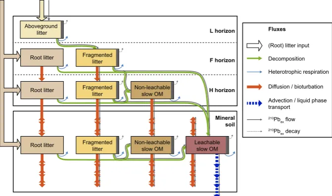
Fig. 1. Overview of the SOMPROF model and the210Pbexmodule. The dark gray rectangles indicate210Pbexassociated with the organic

matter pools.

study went beyond simply reducing the uncertainty ranges of the parameters. We also sought to gain qualitative under-standing of the model’s behavior, specifically its potential ability to explain observations by different mechanisms, and the value of210Pbexdata and prior knowledge to improve pa-rameter identification. This work also represents a first step towards testing the validity of SOMPROF for different soils and ecosystems.

We aim to answer the following questions: (i) what is the relative importance of the different processes involved in SOM profile formation? (ii) How much organic matter is present as material potentially transportable with the liquid phase, as compared to immobile particulate material? And, (iii) are210Pbexprofile measurements useful for constraining the model parameters?

2 Methods

2.1 The SOMPROF model

Here a brief overview of the SOMPROF model is presented. We focus specifically on the model equations in which the estimated parameters are applied, and the210Pbex module. A more exhaustive description and the rationale behind the model structure is presented in Braakhekke et al. (2011).

In SOMPROF the soil profile is divided into the mineral soil and the surface organic layer, which is assumed to con-tain no mineral material and is further subdivided into three horizons: L, F and H (Fig. 1). These organic horizons are simulated as homogeneous connected reservoirs of organic matter (OM). Decomposition products of litter generally flow from the L to the F horizon and from the F to the H

hori-zon. Additionally, material may be transported downward be-tween the organic horizons and into the mineral soil by bio-turbation. For the mineral soil, which comprises both organic matter and mineral material, the model simulates the verti-cal distribution of the organic matter pools, with a diffusion-advection model.

In view of the low rates of the relevant processes, and lack of knowledge of initial conditions at the sites, the SOM-PROF simulations in this study covered the complete period of SOM profile formation, starting without any organic car-bon in the profile. The model was run with a time step length of one month (1/12 yr), for a specified maximum number of years, depending on the age and history of the site, and was driven by repeated annual cycles of measured or esti-mated soil temperature, moisture and (root) litter production. The main reason for considering temperature and moisture was to remove effects of local climate from the estimated decomposition rate coefficients, which thus are more intrin-sic quantities, influenced mostly by local soil and vegetation properties. Furthermore, seasonal fluctuations of the forcing variables were accounted for since the timing of oscillations may have effects on long time scales due to non-linear in-teractions in the model. We limited the forcing cycle to one year, because inter-annual variability is expected to be small compared to seasonal fluctuations and the available measure-ments were not sufficient to derive longer cycles.

2.1.1 Organic matter pools and decomposition

(RL), non-leachable slow organic matter (NLS), and leach-able slow organic matter (LS). Aboveground and root litter receive external input; fragmented litter and leachable and non-leachable slow OM are formed by decomposition. LS is absent in the organic horizons since the adsorptive capac-ity there is assumed to be negligible compared to that of the mineral soil.

Organic matter decomposition is simulated as a first-order decay flux, corrected for soil temperature and moisture. For any organic matter pooli, the decomposition fluxLi is de-fined as:

Li=f (T ) g (W ) kiCi, (1)

whereCi is the concentration (kg m−3, for the mineral soil) or the stock (kg m−2_{, for the organic horizons), k}

i the de-composition rate coefficient (yr−1_{) at 10}◦_{C and optimal soil}

moisture, andf (T )andg(W )the response functions for soil temperature and moisture (see Braakhekke et al., 2011). To avoid errors due to smoothing of the temperature and mois-ture data to monthly values, the response factors were cal-culated for the unsmoothed, daily measurements. These re-sponse factors were subsequently averaged to monthly val-ues, and several years of data were averaged to an average annual cycle, which was used to calculate the decomposition fluxes.

The formation of fragmented litter, non-leachable, and leachable slow OM is defined according to a transformation fraction (αi→j) that determines the decomposition fluxFi→j from donor poolito the receiving poolj:

Fi→j=αi→jLi. (2)

The organic matter that does not flow to other pools is as-sumed to be lost as CO2.

For the calibration measured organic carbon amounts were always compared to total simulated organic carbon, summed over all pools. Mass fraction in the mineral soil layers was calculated as the organic carbon mass divided by the total mass (mineral plus organic) in each layer. Effective decom-position rate coefficients were determined by dividing the to-tal simulated heterotrophic respiration by the toto-tal organic matter stock of the respective layers.

2.1.2 Organic matter transport

All organic matter pools except aboveground litter are trans-ported by bioturbation at equal rate. Conversely, only the leachable slow organic matter pool is transported by liquid phase transport. All transport parameters are assumed con-stant and independent of depth, although the diffusivity of organic matter may vary with depth due to bulk density vari-ations (see Eq. 4).

For the organic layer, organic matter transport due to bioturbation is determined by the bioturbation rate B

(kg m−2yr−1), which represents the mixing activity of the

soil fauna, i.e., the amount of material being displaced per unit area and unit time. B is the maximum flux of organic matter that can be moved to the next horizon. In case the po-tential bioturbation flux for one time step exceeds the amount of organic matter in a horizon, it is adjusted downward. For the mineral soil, a diffusion model is applied to simulate transport due to bioturbation:

∂Ci

∂t

BT

=DBT

∂2Ci

∂z2 , (3)

whereCi is the local concentration of organic matter pooli (kg m−3),zdepth in the mineral soil (m, positive downward;

z=0 at the top of the mineral soil), andt time (yr). DBT is the diffusivity (m2yr−1_{), which is derived from the} bio-turbation rate according to mixing length theory, as follows (Braakhekke et al., 2011):

DBT=

1 2

B

ρMSlm, (4)

where is ρMS is the local bulk density (kg m−3), which is depth dependent and can either be set to measured values or calculated by the model. lm is the mixing length (m), which links the bioturbation rate to the diffusivity. The upper boundary condition, at the top of the mineral soil, is deter-mined by the flux of material coming from theHhorizon.

Dissolved organic matter (DOM) is not explicitly repre-sented in SOMPROF. Instead, the combined effects of ad-and desorption ad-and water flow on the concentration profile of the leachable slow organic matter pool are simulated as an effective advection process:

∂CLS

∂t

_LPT

= −v∂CLS

∂z , (5)

where v is the effective organic matter advection rate (m yr−1). Note that the LS pool represents potentially leach-able material; the bulk of this organic matter is in fact immo-bile due to adsorption to the mineral phase. Hence, the LS pool is also transportable by bioturbation.

The upper boundary condition for LS is determined by the total production in the organic layer. For all pools a zero-gradient condition is used for the lower boundary. Hence, only advection of LS can lead to a loss of organic matter by transport.

2.1.3 210Pbexsimulation

M. C. Braakhekke et al.: Modeling the SOM profile using Bayesian inversion 403

(Fig. 1). The modeled210Pbexconcentration profile is con-trolled by atmospheric input, radioactive decay, and organic matter input, decomposition and transport. The210Pbex mod-ule is based on the following assumptions: (i) variations in time of the atmospheric 210Pbex input are negligible; (ii) 210_Pb

ex is input only into the L horizon; (iii) once in the soil, 210Pbex binds immediately and irreversibly to any or-ganic matter pool; (iv)210Pbex“follows” the organic matter to which it is bound through the decomposition and transport processes; and (v) aside from transport,210Pbexis lost only due to radioactive decay, at a fixed rate of 0.0311 yr−1.

Since210Pbexis only input into the L horizon, which con-tains no root litter, no210Pbex is associated with this pool. Furthermore, external input of organic matter as litter has a diluting effect on210Pbex, while loss of organic matter as CO2 leads to an increase of mass fraction. For the organic horizons, the210Pbexfluxes due to organic matter flow (either by transport or transformation to another pool) are calculated by multiplying the flux from a pool by its210Pbexmass frac-tion. For the mineral soil the transport equations are solved separately for210Pbexassociated with the FL, NLS and LS pools.

Since the atmospheric deposition rate of 210Pbex is not generally known, the210Pbexfractions were normalized rela-tive to the fractions at the mineral soil surface for comparison with observations (see Sect. 2.3.2). Thus, the exact input rate is trivial, and was set to 1. Mineral soil210Pbexmass frac-tions, used for comparing with measurements, were calcu-lated as the total210Pbexamount, summed over all organic matter pools, divided by the total mass (mineral plus or-ganic).

2.2 Site descriptions

2.2.1 Loobos

Loobos is a Scots pine (Pinus sylvestris) forest on a well-drained, sandy soil in the Netherlands (52◦100000N, 5◦4403800E). The climate is temperate/oceanic with an aver-age annual precipitation of 966 mm and an averaver-age temper-ature of 10◦C (WUR, Alterra, 2011). The area, which was originally covered by shifting sands, was planted with pine trees in the early 20th century. Currently, the forest floor is covered with a dense understorey of wavy hair grass (De-schampsia flexuosa) that roots primarily in the organic layer. Due to its young age, the soil is classified as Cambic or Hap-lic Arenosol (IUSS Working Group WRB, 2007; Smit, 1999) but shows clear signs of the onset of podzolization. Because of the high content of quartzitic sand (>94 %), the soil is very poor, which is reflected by a low pH (3–4) and nutrient concentrations, and a virtual absence of soil fauna (Emmer, 1995; Smit, 1999). Organic matter is comprised mostly of mor humus in a thick organic layer of circa 11 cm, and or-ganic carbon fractions in the mineral soil are very low.

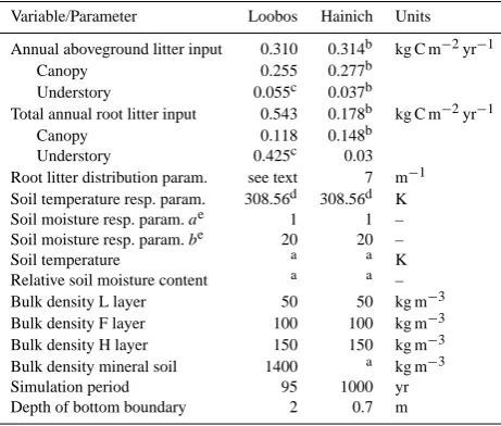
Table 1. Model driving data and not-estimated parameters.

Variable/Parameter Loobos Hainich Units

Annual aboveground litter input 0.310 0.314b kg C m−2yr−1

Canopy 0.255 0.277b

Understory 0.055c _0.037b

Total annual root litter input 0.543 0.178b kg C m−2_yr−1

Canopy 0.118 0.148b

Understory 0.425c 0.03

Root litter distribution param. see text 7 m−1 Soil temperature resp. param. 308.56d 308.56d K Soil moisture resp. param.ae 1 1 – Soil moisture resp. param.be 20 20 –

Soil temperature a a K

Relative soil moisture content a a –

Bulk density L layer 50 50 kg m−3

Bulk density F layer 100 100 kg m−3 Bulk density H layer 150 150 kg m−3 Bulk density mineral soil 1400 a kg m−3

Simulation period 95 1000 yr

Depth of bottom boundary 2 0.7 m

a_{Variable in depth and/or time;}b_{Kutsch et al. (2010); W. Kutsch (personal} communication, 2009);cSmit and Kooijman (2001);dLloyd and Taylor (1994);eSoil moisture response function:g (W )=exp(−exp(a−bW )).

Half-hourly measurements of soil moisture and tempera-ture were performed continuously at five depths (5, 13, 30, 60, 110 cm). Data for the period 1 May 2005 to 31 Decem-ber 2008 were used to derive an average annual cycle of soil temperature and moisture, which was used for the simula-tions. Additionally, aboveground litter fall measurements on a two to four weeks basis for the period 2000 to 2008 were used to derive an average annual cycle for aboveground litter input. Since the carbon content of the litter was not deter-mined, we used a fixed C fraction of 50 %. Bulk density was calculated by the model according to a function from Federer et al. (1993), based on hypothetical bulk densities of pure mineral and pure organic soil (set to 1400 and 150 kg m−3, respectively).

et al. (2007). The root litter input from the canopy vegeta-tion was held constant throughout the simulavegeta-tion. Its ver-tical distribution was also derived from information from Janssens et al. (2002), as well as personal communication from J. Elbers and I. Janssens (2009). At both the Brass-chaat and Loobos sites, it is observed that the root biomass starts at the top of the H horizon and peaks at the mineral soil surface. Therefore, we chose a distribution function that increases linearly with depth from the top to the bottom of the H horizon. From there it decreases with depth according to a two-term exponential function:f (z)=exp(−20.00z)+

0.0384 exp(−0.886z)(see Supplement Fig. 1). By this func-tion we accounted for deep soil input from pine roots, which may be important for the vertical SOM profile. Since the thickness of theH horizon is variable, the total distribution function was normalized at every time step.

The simulation length was set to 95 yr, which is the ap-proximate time between the forest plantation and the sam-pling date. To account for the time needed for vegetation to develop, litter input was reduced in the initial stage, by multi-plying with a function linearly increasing from 0, at the start of the simulation, to 1, after 60 yr (Emmer, 1995).

2.2.2 Hainich

This site is located in the Hainich national park in Central Germany, (51◦4045.3600N, 10◦2707.2000E). The forest, which has been unmanaged for the last 60–70 yr, is dominated by beech (Fagus Sylvatica, 65 %) and ash (Fraxinus excelsior, 25 %) (Kutsch et al., 2010). The forest floor is covered by herbaceous vegetation (Allium ursinum, Mercurialis peren-nis, Anemone nemorosa), which peaks before canopy bud break. The climate is temperate suboceanic/subcontinental with an average annual precipitation of 800 mm and an av-erage temperature of 7–8◦C.

The soil is classified as Luvisol or Cambisol (IUSS Work-ing Group WRB, 2007; Kutsch et al., 2010). It has formed in limestone overlain by a layer of loess, and is character-ized by a high clay content (60 %) and a pH of H2O of 5.9 to 7.8 (T. Persson, personal communication, 2011). The favor-able soil properties support a high biological activity (Cesarz et al., 2007), corroborated by a thin organic layer and a well-developed A horizon. About 90 % of the root biomass occurs above 40 cm depth. A similar distribution was used for the root litter input (Supplement Fig. 1).

The oldest trees at Hainich are approximately 250 yr old, but presumably the site has been covered by similar vegeta-tion for much longer. Thus, we assumed that the soil is close to steady state. Hence, a 1000yr simulation was used. For fur-ther information on the setup of the Hainich simulation, refer to the description of the reference simulation in Braakhekke et al. (2011). The model inputs that were not included in the calibration are listed in Table 1.

2.3 Observations used for the calibration

2.3.1 Organic carbon measurements

For Loobos, measured carbon stocks in the L, F and H hori-zons and the mineral soil, and carbon mass fractions at 3 depths in the mineral profile were used in the calibration. Several profiles were affected by wind erosion; when this was the case, the affected measurements were omitted. In 2005 the soil was sampled in a regular quadratic grid at 25 points spaced 40 m apart. Organic layers were removed with a square metal frame with a side length of 25 cm. The mineral soil was sampled horizon-wise with a P¨urckhauer auger, 2– 3 cm wide and 1 m long. Soil samples were sieved to<2 mm and ground. Carbon stocks in the organic layers were ana-lyzed with a CN analyser Vario EL (Elementar Analysen-systeme GmbH, Hanau, Germany); carbon fractions in the mineral soil were measured with a CN Analyser VarioMax (Elementar Analysensysteme GmbH, Hanau, Germany). For the calibration the mineral soil carbon fractions from differ-ent samplings were interpolated to three fixed depth levels.

For Hainich, measured stocks in the L and F/H horizon (the individualF andHhorizons could not be identified) and in the mineral soil were used, as well as mass fraction mea-surements at 8 depths in the mineral profile. In addition, we used measured effective decomposition rate coefficients at 15◦_{C and soil moisture at 60 % of water holding capacity in}

the L and F/H horizon, and at 7 depths in the mineral profile. The sampling procedure and organic carbon measurements are described in Schrumpf et al. (2011). The decomposition rate coefficients were calculated from measurements of res-piration rates measured during lab incubation of soil sam-ples, which is described in Kutsch et al. (2010). By dividing the average respiration rate of each sample by its organic car-bon content, we obtained effective decomposition rate coef-ficients. All measurements are listed in Supplement Table 1. Simulated organic carbon fractions and effective decom-position rate coefficients were interpolated to the measure-ment depths for comparing with measuremeasure-ments using piece-wise Hermitian interpolation (Burden, 2004). Because or-ganic carbon stocks and mass fractions cannot be less than zero and typically have large spatial variance, the measure-ments from replicate samplings can be assumed to have right-skewed distributions. We assumed that this is also the case for the effective decomposition rate measurements. Therefore, all measurements (and their corresponding model results) were log transformed for the calibration to bring the distribu-tions closer to normal. This also reduced heteroscedasticity for the mineral soil organic carbon fractions.

2.3.2 210Pbexmeasurements

M. C. Braakhekke et al.: Modeling the SOM profile using Bayesian inversion 405

0

5

10

15

20

25

30

35

−0.2 0 0.2 0.4 0.6 0.8

Depth in mineral soil (cm)

210_Pb

ex concentration relative to surface

Hainich Loobos profile 1 Loobos profile 2

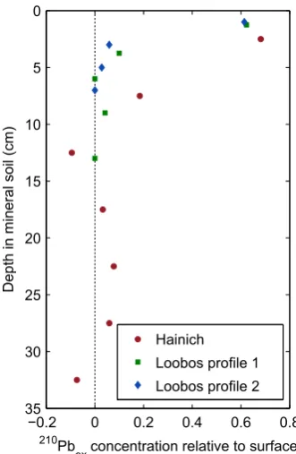
Fig. 2.Measured210_{Pbexconcentrations used for the calibration. Concentrations are relative to the values at}

the surface. Note that the210_{Pbexmeasurements for Loobos are taken from an equivalent site (Kaste et al.,}

2007).

0 1 2 3

Probability

kAGL,kRL,kFL

A

0 0.5 1

kNLS,kLS

B

0 0.5 1 Parameter value

αAGL→FL

C

0 0.5 1

αFL→NLS,αFL→LS,

αRL→NLS,αRL→LS

D

0 upper

bound B,lm,v

E

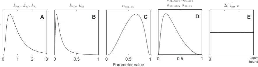
Fig. 3.Prior probability distributions of the model parameters used for calibration setup 3. See Table 2 for the parameters of the distribution functions. All distributions are bounded at zero and an upper bound which are given in Table 2.

35

Fig. 2. Measured210Pbexconcentrations used for the calibration.

Concentrations are relative to the values at the surface. Note that the210Pbexmeasurements for Loobos are taken from an equivalent

site (Kaste et al., 2007).

New Hampshire, USA. This site has conditions similar to those at Loobos in terms of vegetation, soil texture, soil pH, and soil biological activity (Bormann and Likens, 1994). Fur-thermore, pedological processes related to podzol formation are occurring at both sites. The two sites differ with respect to age, since the Loobos soil is very young. However, in view of the relatively fast decay rate of210Pb, and the shallow dis-tribution of the210Pbexprofile (Fig. 2), we assume that it is close to steady state at both sites.

Local210Pbexmeasurements at Hainich were performed for a study by Fujiyoshi and Sawamura (2004) (R. Fujiyoshi, personal communication, 2008). Although these measure-ments were corrected for in situ formed210Pb by subtracting the 226Ra activity (R. Fujiyoshi, personal communication, 2008), the activity profile did not approach zero with depth. Hence, this method did presumably not account for all sup-ported210Pb. Therefore, we assumed that the210Pbex con-centration is zero from approximately 12.5 cm downwards. The supported210Pb activity was estimated as the average below this depth, and all data were corrected by subtracting this average. (Note that in several cases this produced nega-tive concentrations.)

Only mineral soil210Pbexmeasurements were used in the calibration (Fig. 2 and Supplement Table 1). The profiles of both sites, as well as those predicted by the model, were nor-malized by dividing them by the210Pbexactivity at the

sur-face of the mineral soil, which was estimated using piecewise Hermitian extrapolation. Simulated210Pbexfractions and ef-fective decomposition rate coefficients were interpolated to the measurement depths also using Hermitian interpolation, for comparing with measurements. Because of the negative observed values for Hainich, no log-transformations were used for the210Pbexdata.

2.4 Bayesian calibration

We performed Bayesian estimation of 13 model parameters: five decomposition rate coefficients, five transformation frac-tions, and three transport parameters (Table 2). Bayesian cal-ibration is aimed at deriving the posterior probability distri-butionp(θ|O)of the model parametersθbased on the misfit between the model results and the observationsO, and the a priori probability distribution of the parameters (Mosegaard and Sambridge, 2002). According to Bayes’ theorem, the posterior distribution is defined as:

p(θ|O)=c p(θ) p(O|θ), (6)

wherep(θ)is the prior probability distribution, expressing our knowledge of the parameters prior to the calibration, and

cis a normalization constant, ensuring that the integral over the distribution equals 1.p(O|θ)is a likelihood function that expresses the probability of the observations O, given the parametersθ(Gelman et al., 2004, Chap. 1).

The calibrations were performed in three setups, in which 210_Pb

ex data and prior knowledge were stepwise added, in order to investigate the information content of each source of information. For both sites, we ran calibrations in the follow-ing setups:

1. excluding210Pbexdata and with weak priors; 2. including210Pbexdata and with weak priors; 3. including210Pbexdata and with strong priors.

Calibration setup 3 represents our best estimate of the model parameters.

2.4.1 Likelihood function

As discussed in Sect. 2.3, different types of observed vari-ables were used in the calibration, referred to as “data streams”. For any data stream (i), the observations (Oi) may be seen as the sum of the model prediction (Mi(θ)) plus a stochastic residual term (i):

Oi=Mi(θ)+i, i=1,2. . . I. (7)

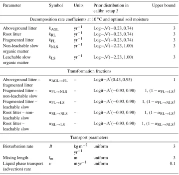
Table 2. The model parameters estimated in the calibration. Note that the prior distributions were only used for calibration setup 3. The lower

bound for all parameters is zero; the upper bound is given in the table.

Parameter Symbol Units Prior distribution in Upper bound calibr. setup 3

Decomposition rate coefficients at 10◦C and optimal soil moisture

Aboveground litter kAGL yr−1 Log−N(−0.23,0.74) 3

Root litter kRL yr−1 Log−N(−0.23,0.74) 3

Fragmented litter kFL yr−1 Log−N(−0.23,0.74) 3

Non-leachable slow kNLS yr−1 Log−N(−2.23,1.00) 3

organic matter

Leachable slow kLS yr−1 Log−N(−2.23,1.00) 3

organic matter

Transformation fractions

Aboveground litter – α_AGL→FL – Logit−N(0.43,0.95) 1

fragmented litter

Fragmented litter – αFL→NLS – Logit−N(−0.93,0.98) 1,(1−αFL→LS)

non-leachable slow

Fragmented litter – αFL→LS – Logit−N(−0.93,0.98) 1,(1−αFL→NLS)

leachable slow

Root litter – non- αRL→NLS – Logit−N(−0.93,0.98) 1,(1−αRL→LS)

leachable slow

Root litter – αRL→LS – Logit−N(−0.93,0.98) 1,(1−αRL→NLS)

leachable slow

Transport parameters

Bioturbation rate B kg m−2 uniform 3

yr−1

Mixing length lm m uniform 3

Liquid phase transport v m yr−1 uniform 0.1 (advection) rate

conditional likelihood function for a givenσi is defined by the joint distribution of the residuals of all data streams:

p(O|θ,σ2)∝

I

Y

i=1

σ−Ni

i exp −

1

2σ_i2SSi(θ)

!

. (8)

Note that we did not consider correlations between the dif-ferent variables. SSi(θ)is the sum of squared residuals for data stream (i) over all (Ni) data points:

SSi(θ)=

Ni X

n=1

(Oi, n−Mi, n(θ))2. (9)

Multiple replicate measurements, if available, were all indi-vidually included in Si(θ), meaning a single model predic-tion was compared to multiple observapredic-tions. For the mineral soil profile, measurements from all depth levels were con-sidered to be part of the same data stream; i.e., the residuals were assumed to have the same distribution.

The variance of the residuals(σ_i2)is usually determined by both model-related errors (deficiencies in the model

struc-ture, errors in forcing data) as well as observational uncer-tainty (spatial heterogeneity, measurement errors). In some cases it may be estimated a priori based on knowledge of the model and the measurement uncertainty (Knorr and Kattge, 2005), but in general it must be considered unknown. For certain prior distributionsσi can be analytically integrated out of the joint likelihood functionp(O,σ2_{|θ), yielding the}

marginal distribution(p(O|θ); Gelman et al., 2004, Chap. 3). We use the uninformative prior p(σi)∝1/σi, which yields the following formulation of the likelihood function:

p(O|θ)_∝

I

Y

i=1

SSi(θ)−Ni/2. (10)

2.4.2 Prior parameter distributions

M. C. Braakhekke et al.: Modeling the SOM profile using Bayesian inversion 407

0

5

10

15

20

25

30

35

−0.2

0

0.2

0.4

0.6

0.8

Depth in mineral soil (cm)

210

_Pb

ex

concentration relative to surface

Hainich

Loobos profile 1

Loobos profile 2

Fig. 2. Measured210Pbexconcentrations used for the calibration. Concentrations are relative to the values at

the surface. Note that the210Pbex measurements for Loobos are taken from an equivalent site (Kaste et al.,

2007).

0 1 2 3

Probability

kAGL,kRL,kFL

A

0 0.5 1

kNLS,kLS

B

0 0.5 1

Parameter value

αAGL→FL

C

0 0.5 1

αFL→NLS,αFL→LS,

αRL→NLS,αRL→LS

D

0 upper

bound

B,lm,v

E

Fig. 3.Prior probability distributions of the model parameters used for calibration setup 3. See Table 2 for the

parameters of the distribution functions. All distributions are bounded at zero and an upper bound which are

given in Table 2.

35

Fig. 3. Prior probability distributions of the model parameters used for calibration setup 3. See Table 2 for the parameters of the distribution

functions. All distributions have a lower bound at zero and an upper bound which is given in Table 2.

For the runs with strong priors, the distributions were based on knowledge from previously published studies (Braakhekke et al., 2011). The same distributions were used for both sites. Since decomposition rate coefficients cannot be negative or zero, we chose a log-normal distribution. For the litter pools (kAGL,kRLandkFL), we used the same distri-butions (mode at 0.46 yr−1_{; Fig. 3a). It is likely that the} de-composition rate coefficient of leachable slow organic matter (kLS) is lower than that of non-leachable slow organic matter (kNLS), since the former is comprised mostly of material ad-sorbed to the mineral phase. Nevertheless, since we aimed to test this hypothesis with the measurements, we used the same prior distributions for the decomposition rate coefficient of both pools (mode at 0.04 yr−1; Fig. 3b).

We used logit-normal prior distributions for the transfor-mation fractions. This distribution is similar to the beta dis-tribution and is bounded between 0 and 1 (Mead, 1965). ForαAGL→FL a distribution with the mode at 0.68 was used (Fig. 3c), while for the other conversion fractions (αRL→NLS,

αRL→LS, αFL→NLS, and αFL→LS) the same prior was used with the mode at 0.18 (Fig. 3d). Since relatively little a pri-ori information about the SOM transport parameters (B,lm, andv) is available, we used uniform priors for all calibrations (Fig. 3e).

For all calibration setups, the sampling was constrained to a bounded region in parameter space. This constraint was included since preliminary runs showed that some parame-ters may be unconstrained at the upper bound by the data, due to over-parameterization. The lower bounds for all pa-rameters were set to zero; the upper bounds are listed in Table 2. Additionally, since decomposition must not lead to a net formation of material, the sum of transformation frac-tion for root litter (αRL→NLS+αRL→LS) and fragmented litter (αFL→NLS+αFL→LS) pools was bounded to 1.

2.4.3 Monte Carlo simulations

The complexity of SOMPROF precludes analytical model in-version or expression of the normalizing constant in Eq. (6). Therefore, we approximated the posterior distribution using

a Markov chain Monte Carlo algorithm. Such algorithms obtain a sample of the posterior distribution by perform-ing a random walk through parameter space. They are in-creasingly used for calibrating ecosystem models against eddy-covariance measurements and satellite data (Knorr and Kattge, 2005; Fox et al., 2009) and have been applied to cal-ibrate soil carbon models as well (Yeluripati et al., 2009; Scharnagl et al., 2010; de Bruijn and Butterbach-Bahl, 2010). We used the Metropolis algorithm DREAM(ZS) (Laloy and Vrugt, 2012), a successor to DREAM (Vrugt et al., 2009), which has been shown to perform well for complex, multi-modal distributions . Further information concerning the cal-ibration setup can be found in Appendix A1.

3 Results

3.1 Loobos

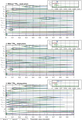
Figure 4 depicts the marginal posterior distributions for the three calibrations for Loobos (see also Supplement Table 2). For calibration setups 1 and 2, several parameters have wide distributions compared to the sampling range, which shows they are poorly constrained by the observations. Furthermore, for some of the parameters (kRL, αFL→LS,

αRL→NLS, lm, and v) the highest density point appears to lie at or near the upper or lower bound. Adding210Pbex im-proved the constraint of the bioturbation-related parameters (Bandlm) but had otherwise no major effect on the marginal distributions. Inclusion of prior knowledge reduced uncer-tainty, particularly for the parameters that are poorly con-strained by the data.

The results of the forward simulations (Fig. 5a, additional results shown in Supplement Fig. 4) indicate that leach-able slow organic matter (LS) is the most abundant pool, followed by non-leachable slow organic matter (NLS). LS particularly dominates the mineral soil, being virtually the only pool below 20 cm. Figure 5b shows that most organic matter in the mineral soil is derived from root litter, but aboveground-derived SOM is present up to great depths, due to fast downward migration by liquid phase transport. Fig-ure 6a shows the organic matter transport fluxes in the min-eral soil. Clearly, transport due to bioturbation plays almost no role; virtually all transport occurs by movement with the liquid phase. Figure 6b, which depicts the amount of organic carbon in the steady state derived from the three processes, corroborates the importance of liquid phase transport. The negative concentrations for this process indicate it causes or-ganic matter from near the surface – mainly root litter de-rived – to be moved downward to greater depths, where it is the dominant mechanism of input.

3.2 Hainich

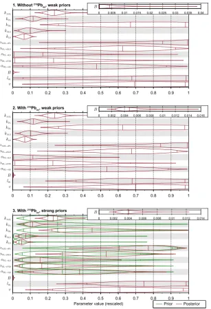
For Hainich, the posterior distribution is multi-modal for all calibration setups, comprising three distinct optima. For analysis, the modes were sampled individually in separate calibration runs. An additional calibration run was performed in which all modes were sampled simultaneously to assure that the multi-modality is not an artifact of the sampling (see Supplement Fig. 3). The marginal distributions for all cali-bration setups and all modes are depicted in Fig. 7 (see also Supplement Table 2). While the distributions of most param-eters differ between the modes, the most prominent differ-ences can be seen for the decomposition rate coefficients of root litter (kRL), non-leachable slow (kNLS), and leachable slow (kLS) organic matter. For each of the modes, one of these three parameters is tightly constrained at the low end of the range, while the other two have wide distributions at higher values.

Addition of210Pbexto the observations caused shifts and re-duction of uncertainty for some parameters (e.g.,vfor mode A,lm for mode B), but had in general no major effects on the posterior. Changing from weak to strong priors reduced uncertainty for parameters that are poorly constrained by the observations.

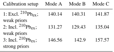
The comparative probability of the modes cannot be in-ferred from Fig. 7, since the distributions are scaled to the same height. To compare the modes we introduce the “misfit”

S(θ)as the negative logarithm of the unnormalized posterior density (Mosegaard and Sambridge, 2002):

S(θ)= −ln(p(θ) p(O|θ))= −ln(p(θ))− I X

i=1

ln(SSi(θ)) , (11)

where SSi(θ)is defined according to Eq. (9). A lower mis-fit indicates a higher posterior density and a better mis-fit to the observations and priors. Note that the contribution of a sin-gle data stream toS(θ)may be negative for a high fit and/or small Ni. The modes are compared according to the low-est misfit in the calibration samples (Table 3). This shows that the three calibrations setups differ notably in terms of the comparative probability of the modes. In calibration 1 the three modes have similar misfit. Introduction of210Pbex and prior information to the calibration caused the misfit of mode C to increase markedly compared to A and B, which is explained by a somewhat poorer fit to the210Pbex measure-ments (results not shown), as well as the very low root lit-ter decomposition rate coefficient, which conflicts with prior knowledge.

M. C. Braakhekke et al.: Modeling the SOM profile using Bayesian inversion 409

kAGL kFL kRL kNLS kLS αAGL→FL αFL→NLS αFL→LS αRL→NLS αRL→LS B lm

v

0 0.1 0.2 0.3 0.4 0.5 0.6 0.7 0.8 0.9 1

B

0 0.005 0.01 0.015 0.02 0.025 0.03 0.035 0.04

1. Without 210_Pb

ex, weak priors

kAGL kFL kRL kNLS kLS αAGL→FL αFL→NLS αFL→LS αRL→NLS αRL→LS B lm

v

0 0.1 0.2 0.3 0.4 0.5 0.6 0.7 0.8 0.9 1

B

0 0.002 0.004 0.006 0.008 0.01 0.012 0.014 0.016

2. With 210_Pb

ex, weak priors

Parameter value (rescaled)

kAGL kFL kRL kNLS kLS αAGL→FL αFL→NLS αFL→LS αRL→NLS αRL→LS B lm

v

0 0.1 0.2 0.3 0.4 0.5 0.6 0.7 0.8 0.9 1

Prior Posterior

B

0 0.002 0.004 0.006 0.008 0.01 0.012 0.014

3. With 210_Pb

ex, strong priors

Fig. 4.

Posterior distributions for the three setups for Loobos. The “violins” depict the marginal distribution for

each parameter. The three vertical lines inside the violins indicate the median and the 95 % confidence bounds.

The parameters are normalized to the sampling ranges (see Table 2).

Fig. 4. Posterior distributions for the three setups for Loobos. The “violins” depict the marginal distribution for each parameter. The three

vertical lines inside the violins indicate the median and the 95 % confidence bounds. The parameters are normalized to the sampling ranges (see Table 2).

However, they represent an important mechanism for mov-ing organic matter from shallow levels to deeper layers, as indicated by the negative values near the surface.

4 Discussion

4.1 Loobos

The calibration results for Loobos suggest that leachable slow (LS) OM is the most abundant organic matter fraction. Its transport with the liquid phase, representing dissolved

or-ganic matter leaching, is largely responsible for downward SOM movement and formation of the vertical SOM profile in general. Although the decomposition rate coefficient of this pool (kLS) is the lowest, its distribution tends to quite high values (optimum approximately 0.189 yr−1 in calibra-tion setup 3; Fig. 4c; Supplement Table 2). Particularly con-sidering that LS is the only pool in the deep soil, where de-composition is slow, we would expect a lower value forkLS. The prior distribution of this parameter used in calibration setup 3, which tends to lower values, caused only a slight downward shift in the posterior. Due to its large variance, the

0 0.5 1 1.5 2

C stock (kg m

−2)

(a) Soil organic matter pools

L

F H

top soil subsoil

Depth in mineral soil (cm)

C mass fraction (%) 20

40

60

80

0 0.5 1 1.5

Aboveground litter Fragmented litter Root litter Non−leachable slow OM Leachable slow OM Measured C stock Measured C fraction

± 1 SD mod. C fraction

0 0.5 1 1.5 2

(b) Above/belowground derived soil organic carbon

L

F H

top soil subsoil

C mass fraction (%) 20

40

60

80

0 0.5 1 1.5

Abovegr. litter derived Root litter derived Measured C stock Measured C fraction

± 1 SD mod. C fraction

Fig. 5. Organic carbon measurements and corresponding model

re-sults of forward Monte Carlo simulations for Loobos, based on pos-terior distribution of calibration setup 3. (a) Stocks and fractions of the model pools; (b) above- vs. belowground derived organic mat-ter. L, F, and H refer to the organic horizons (see Sect. 2.1); topsoil: 0–30 cm; subsoil:>30 cm; OM: organic matter. All model results are averages over the Monte Carlo ensemble; error bars denote one standard error of the mean for the measurements and one standard deviation (SD) for the model results.

Table 3. Minimum misfit value (see Eq. 11) in the posterior sample

for each of the modes for Hainich for the three calibration setups. Note that the misfit values of calibration setup 2 are lower than those of calibration setup 1. This is caused by the fact that the misfit values for the210Pbex are negative due to the small number of data points (cf. Eq. 10).

Calibration setup Mode A Mode B Mode C 1: Excl.210Pbex; 140.14 140.31 141.87

weak priors

2: Incl.210Pbex; 131.27 129.43 135.04

weak priors

3: Incl.210Pbex; 146.56 142.9 157.57

strong priors

posterior distribution ofkLSdoes allow for somewhat lower, more realistic values. Furthermore, there are quite strong cor-relations between parameters related to the LS pool (Supple-ment Fig. 6), which indicate that a decrease of the formation of LS (determined byαFL→LSandαRL→LS) can be compen-sated by a decrease of the liquid phase transport ratevor the decomposition rate coefficientkLS, both controlling the loss of this pool.

Although SOMPROF was not developed to simulate dis-solved organic matter transport, the modeled liquid phase transport fluxes should represent the average movement of

Depth in mineral soil (cm)

Transport flux (kgC m−2 _yr−1₎ (a) Soil organic carbon transport

0

20

40

60

80

100

120

0 0.1 0.2 0.3

Bioturbation Liquid phase transport

±1 standard deviation

Measured DOC flux

Concentration (kg m−3₎ (b) Contribution of processes

to soil organic carbon

0

10

20

30

40

50

60

70

−10 0 10 20

Root litter input Bioturbation Liquid phase transport

±1 standard deviation

30

40

50

60

70

0 1 2

Fig. 6. Simulated organic carbon fluxes from forward Monte Carlo

simulations for Loobos, based on posterior distribution of calibra-tion setup 3 (note the different scales on the y-axes). All quantities are averages over the last simulation year and the Monte Carlo en-semble. (a) Organic carbon transport fluxes and measured dissolved organic carbon (DOC) fluxes (Kindler et al., 2011; not used in the calibration). Note the indistinct bioturbation flux in the upper left corner. (b) Contributions of the different processes to soil organic matter profile in mineral soil (see Sect. 2.4.3).

dissolved organic carbon (DOC) over long timescales1_. Fig-ure 6a shows that simulated liquid phase transport fluxes are an order of magnitude higher than DOC fluxes measured by Kindler et al. (2011), which points to a too high value of the advection ratev. However, the high uncertainty of both the rate and fluxes of liquid phase transport shows that the ob-servations used in the calibration can also be explained with somewhat lower values. A lower value forv would be ac-companied by a lower decomposition rate coefficient of LS, since the two parameters are strongly correlated (Supplement Fig. 6). Thus, it is likely that additional observations con-straining the deep soil decomposition rate coefficient, such as radiocarbon measurements, would lead to a more realistic estimate of liquid phase transport rate.

Notwithstanding the over-estimated liquid phase transport fluxes, the relative importance of organic matter leaching over bioturbation is in good agreement with the soil condi-tions and humus form at Loobos. Soil fauna is virtually ab-sent, and the high concentration of sand supports fast water infiltration and has a low adsorptive capacity, thus allowing high dissolved organic matter fluxes.

1_{While the LS pool represents mostly material adsorbed to the}

M. C. Braakhekke et al.: Modeling the SOM profile using Bayesian inversion 411

1. Without 210_Pb

ex, weak priors

kAGL kFL kRL kNLS kLS αAGL→FL αFL→NLS αFL→LS αRL→NLS αRL→LS B lm

v

0 0.1 0.2 0.3 0.4 0.5 0.6 0.7 0.8 0.9 1

kRL kNLS kLS v

0 0.005 0.01 0.015 0.02 0.025 0.03

2. With 210_Pb

ex, weak priors

kAGL kFL kRL kNLS kLS αAGL→FL αFL→NLS αFL→LS αRL→NLS αRL→LS B lm

v

0 0.1 0.2 0.3 0.4 0.5 0.6 0.7 0.8 0.9 1

kRL kNLS kLS v

0 0.005 0.01 0.015 0.02 0.025 0.03

Parameter value (rescaled)

3. With 210_Pb

ex, strong priors

kAGL kFL kRL kNLS kLS αAGL→FL αFL→NLS αFL→LS αRL→NLS αRL→LS B lm

v

0 0.1 0.2 0.3 0.4 0.5 0.6 0.7 0.8 0.9 1

kRL kNLS kLS v

0 0.005 0.01 0.015 0.02 0.025 0.03

Mode A Mode B Mode C

Fig. 7.

Posterior distributions for the three calibration setups for Hainich. The “violins” depict the marginal

distribution for each parameter. The three posterior modes are plotted separately in the same graph. The

three vertical lines inside the violins indicate the median and the 95 % confidence bounds. The parameters are

normalized to the sampling ranges (see Table 2).

Fig. 7. Posterior distributions for the three calibration setups for Hainich. The “violins” depict the marginal distribution for each parameter.

The three posterior modes are plotted separately in the same graph. The three vertical lines inside the violins indicate the median and the 95 % confidence bounds. The parameters are normalized to the sampling ranges (see Table 2).

4.2 Hainich

The presence of multiple modes in the posterior distribu-tions for Hainich is illustrative of the equifinality problem discussed in the introduction. Since the modes represent sep-arate isolated regions in parameter space, they may be seen as distinct explanations for the observations, in terms of the processes represented in the model. In calibration setup 1 the

three modes have similar misfits (Table 3). The addition of 210_Pb

exto the calibration leads to a shift in the comparative misfit, causing mode B to become dominant. Switching to strong priors further increased these differences. Based on these results we can discard mode C with some certainty. The difference between modes A and B, however, is rela-tively small. Hence, in view of unconsidered uncertainties

(a) Soil organic matter pools

0 5 10 15

C stock (kg m

−2)

Mode A

L F H F+H top soil

sub soil

Depth in mineral soil (cm)

20

40

60

0 2 4 6 8 10 12 0 5 10

15 Mode B

L F H F+H top soil

sub soil

C mass fraction (%) 20

40

60

0 2 4 6 8 10 12 Aboveground litter Fragmented litter Root litter

Non−leachable slow OM Leachable slow OM

Measured C stock Measured C fraction

± 1 SD mod. C fraction

0 5 10

15 Mode C

L F H F+H top soil

sub soil

20

40

60

0 2 4 6 8 10 12

(b) Above/belowground derived soil organic carbon

0 5 10 15

C stock (kg m

−2)

Mode A

L _{F H F+H}

top soil

sub soil

Depth in mineral soil (cm)

20

40

60

0 2 4 6 8 10 12

0 5 10

15 Mode B

L F H F+H

top soil

sub soil

C mass fraction (%) 20

40

60

0 2 4 6 8 10 12

Abovegr. litter derived Root litter derived Measured C stock Measured C fraction ± 1 SD mod. C fraction

0 5 10

15 Mode C

L F H F+H

top soil

sub soil

20

40

60

0 2 4 6 8 10 12

Fig. 8. Organic carbon measurements and corresponding model results of forward Monte Carlo simulations for Hainich, based on the three

posterior modes of calibration setup 3. (a) Stocks and fractions of the model pools; (b) above- vs. belowground derived organic matter. L, F, and H refer to the organic horizons (see Sect. 2.1); topsoil: 0–30 cm; subsoil:>30 cm; OM: organic matter. All model results are averages over the Monte Carlo ensemble; error bars denote one standard error of the mean for the measurements and one standard deviation (SD) for the model results.

(see Sect. 4.6) we cannot fully ignore mode A as possible explanation for the observations.

Figure 9a shows that for all modes the modeled advective flux is substantially larger than the DOC fluxes measured by Kindler et al. (2011). However, for mode B the overestima-tion is less pronounced, particularly in the subsoil. For modes A and C, modeled advective flux and its uncertainty are very high. Contrastingly, the contribution of advection to input in the profile is very small and well constrained for both modes (Fig. 9b). The reason is that the advective fluxes have rel-atively small vertical gradients. This also explains the high uncertainty of the advective flow (and the advection ratev) for these modes: as long as its gradient does not change, the actual flux can vary relatively freely.

The abundance of LS and the low rate of liquid phase transport for mode B agrees well with expectations based on the soil texture at Hainich. The high clay content

im-pedes water infiltration, while favoring adsorption of organic matter, slowing down both dissolved organic matter leach-ing and decomposition of organic matter. This is corrobo-rated by organic matter density fractionation measurements at the site (Schrumpf, 2011). These indicate that 81–93 % of the organic matter is present in the heavy fraction, which is known to comprise mostly material in organo-mineral com-plexes (Golchin et al., 1994). Although the model pools can presumably not be compared directly to the measured density fractions, this is clearly in support of mode B, since leach-able slow OM represents mostly material adsorbed to the mineral phase (Sect. 2.1.2; Braakhekke et al., 2011). Based on these arguments, we conclude that mode B represents the most likely explanation for the observations at Hainich.

M. C. Braakhekke et al.: Modeling the SOM profile using Bayesian inversion 413

(a) Soil organic carbon transport

Mode C 0

10

20

30

40

50

60

70

80

0 0.02 0.04 0.06 0.08

Depth in mineral soil (cm)

Mode A 0

10

20

30

40

50

60

70

80

0 0.02 0.04 0.06 0.08

Transport flux (kgC m−2 _yr−1₎

Mode B 0

10

20

30

40

50

60

70

80

0 0.02 0.04 0.06 0.08

Bioturbation Liquid phase transport.

±1 standard deviation Measured DOC flux

(b) Contribution of processes to soil organic carbon

Depth in mineral soil (cm)

Mode A 0

10

20

30

40

50

60

70

−20 0 20 40 60 80

30

40

50

60

70

80

0 5 10

Mode C 0

10

20

30

40

50

60

70

−20 0 20 40 60 80

30

40

50

60

70

80

0 5 10

Concentration (kg m−3₎ Mode B 0

10

20

30

40

50

60

70

−20 0 20 40 60 80

Root litter input Bioturbation Liquid phase transport

±1 standard deviation 30

40

50

60

70

80

0 5 10

Fig. 9. Simulated organic carbon fluxes from forward Monte Carlo simulations for Hainich, based on the three modes of the posterior

distribution of calibration setup 3 (note the different scales on the y-axes). All quantities are averages over the last simulation year and the Monte Carlo ensemble. (a) Organic carbon transport fluxes and measured dissolved organic carbon (DOC) fluxes (Kindler et al., 2011; not used in the calibration); (b) contribution of the different processes to soil organic matter profile in mineral soil (see Sect. 2.4.3).

fraction, its decomposition products (mainly LS) constitute the bulk of the total SOM. The effects of the transport pro-cesses are generally small compared to material derived from root litter input. However, particularly advection causes loss of material near the surface, and input into deeper layers. The relative importance of root-derived SOM agrees well with re-cent findings by Tefs and Gleixner (2012), who found, based on 14C profile measurements, that soil organic carbon dy-namics at Hainich are mainly determined by root input.

4.3 Comparison between sites

It is difficult to explain why the posterior distributions for Loobos do not display multi-modality, like the distributions for Hainich. One possible explanation is the fact that the ob-served mineral soil C profile for Loobos clearly consists of two zones: one with a fast decrease with depth between 0 and 10 cm, and one below this, with a much slower decrease. It is

conceivable that such a profile can only be explained by a sit-uation where diffusion (bioturbation) operates only near the surface, while advection (liquid phase transport) acts in the complete profile. For Hainich, on the other hand, the C pro-file is smoother, thus allowing it to be explained by different mechanisms.

decomposition rates of the pools that dominate there. Com-parison further shows that the decomposition rate coefficient of the main pool LS is markedly lower for Hainich, and much less uncertain. This is presumably explained by the observa-tions of the effective decomposition rate coefficients. For the deep soil these data directly constrain the decomposition rate coefficient of LS since this is virtually the only pool there (see also Supplement Fig. 5). In view of the considerable ef-fort involved with such measurements, a study into the value of such data for inferring SOMPROF parameters would be valuable. However, in general care must be taken when us-ing lab measurements to infer parameters for field condi-tions. Furthermore, for the decomposition rate coefficients of the slow pools, very long incubation times may be required (Scharnagl et al., 2010).

The two sites differ strongly with respect to the organic matter transport parameters, with Hainich having a higher bioturbation rate, and Loobos having a higher liquid phase transport rate. This is in good agreement with the differences between the two sites in terms of biological activity and soil texture.

4.4 Implications for soil organic matter cycling

The fact that leachable slow organic matter pool constitutes the bulk of SOM for both sites emphasizes the importance of organo-mineral interactions for soil carbon cycling. How-ever, this interpretation relies on the assumption that mineral-associated organic matter is correctly represented by the LS pool. Mathematically, the only difference between the NLS and LS pools lies in the transport behavior: diffusion-only versus diffusion and advection. The question is whether this distinction correctly represents the differences between sta-ble particulate and adsorbed organic matter in reality. The good agreement of our results with density fractionation measurements at Hainich, as well as the environmental con-ditions at both sites, suggests that an explanation where LS dominates might indeed be appropriate. Furthermore, many studies have demonstrated the importance of mineral asso-ciations for long-term carbon preservation (Eusterhues et al., 2003; Mikutta et al., 2006; K¨ogel-Knabner et al., 2008; Kalb-itz and Kaiser, 2008). In contrast, others have indicated the presence of root-derived particulate material in podzol B horizons, and questioned the relevance of mineral-associated material for mineral soil organic matter fractions (Nierop, 1998; Nierop and Buurman, 1999; Buurman and Jongmans, 2005).

The predominance of root-derived material predicted for both sites (Figs. 5 and 8, mode B) underlines the importance of roots for organic matter input in the mineral soil, which is in agreement with previous studies (Kong and Six, 2010; Rasse et al., 2005). For Hainich, the root input also strongly determines the vertical distribution of SOM (Fig. 9), whereas for Loobos also redistribution of organic material by liquid phase transport is a major factor (Fig. 6). Based on

analy-sis of a large database of SOM profiles, Jobbagy and Jack-son (2000) found that root/shoot allocation, together with the root biomass distribution, explains the vertical SOM profile in the upper part of the soil while clay content was found to be more important at greater depths. The effects of texture are not considered in this study, but Figs. 6b and 9b show that the relative importance of liquid phase transport becomes greater with depth. This supports the findings of Jobbagy and Jack-son (2000) since this mechanism is likely strongly controlled by soil texture.

4.5 The use of210Pbexmeasurements

The addition of210Pbexto the calibration had no major ef-fects on the posterior distributions. For Loobos, the210Pbex measurements improved the constraint of the parameters re-lated to bioturbation, while for Hainich they improved con-straint of the mixing length for mode B, and caused an in-crease of the misfit of mode B and C relative to mode A. The fact that the210Pbexdata influenced only parameters re-lated to bioturbation may be explained by the fact that the profiles used here are quite shallow, due to the relatively fast decay rate of the isotope (cf. Fig. 2). These measurements are therefore presumably most informative for the topsoil, where bioturbation is more important.

For both sites, the measured210Pbex profile was already well matched by the model in calibration setup 1, in which these measurements were not included. This indicates that these observations can be explained well in conjunction with the organic carbon measurements, which supports the model structure. It also suggests that the210Pbex data from Kaste et al. (2007) are consistent with the conditions at Loobos.

M. C. Braakhekke et al.: Modeling the SOM profile using Bayesian inversion 415

while movement of dissolved Pb2+_{was found to be}

unimpor-tant (Wang and Benoit, 1997).

In summary, further study on this topic is needed, but we believe that use of 210Pbex as a tracer for SOM transport is well defendable. Despite the limited constraint gained in this study, this isotope can be useful as a tracer for SOM transport, provided that more replicate measurements are available to reduce uncertainty. Particularly in combination with other tracers, such as14C or137Cs,210Pbexmay be quite informative.

4.6 Methodological constraints and model validity

For both sites, many strong correlations exist between differ-ent combinations of model parameters (Supplemdiffer-ent Fig. 6), which indicates that the model is over-parameterized with re-spect to the available data. Furthermore, for all calibration setups there is at least one decomposition rate coefficient for which high values are not constrained by the observa-tions (Figs. 4 and 7). Since the predicted stock of a pool is inversely proportional to its decomposition rate coefficient, these pools are present in very small amounts, which shows that SOMPROF has at least one redundant organic matter pool, given the available data. This is further demonstrated by a strong negative correlation between decomposition rate coefficient of FL and RL for Loobos (Supplement Fig. 6), indicating that these pools are essentially “competing” as ex-planation for the observed carbon stocks and fractions. In order to obtain better constraint, additional observations are needed. Obvious candidates for such data are carbon isotopes (13C or14C) measurements, of both organic matter and het-erotrophic respiration.

There are numerous uncertainties that were not consid-ered in the calibration. In view of practical limitations on the number of parameters that can be estimated simultane-ously, we focused on the inherently unmeasurable parame-ters, on which little prior information was available. Many other model inputs, with varying degrees of uncertainty, were held fixed, including the temperature and moisture data, the litter input rates, and the temperature and moisture response parameters. Another source of uncertainty is associated with site history. The sites included in this study were selected for having a relatively well-known and constant history, but par-ticularly for Hainich there have undoubtedly been past fluc-tuations in the forcing that were not considered. Finally, con-siderable uncertainty is related to the model structure, specif-ically to the simple representations of organic matter decom-position and transport in SOMPROF as well as the behav-ior of210Pbex. These unconsidered variabilities call for care when interpreting the results. Further, it may be advisable to inflate the variance of the posterior distributions when using them as priors for a follow-up study, or for predictive simula-tions. Nevertheless, we believe that the parameters that were estimated constitute the most important uncertainties.

The good fit to the observations indicates that SOMPROF is able to reproduce widely different SOM profiles, based on realistic parameter values. Furthermore, the consistency of the results with site conditions and the good fit to the210Pbex measurements (even when they are not included in the cal-ibration) are encouraging and support the validity of SOM-PROF for temperate forests. The validity for other ecosys-tems such as grasslands and tropical and boreal forests is yet to be established. Also, comparison to other types of mea-surements is needed, both to improve constraint of the pro-cesses, and to further evaluate the model. Examples of such data include carbon isotopes, heterotrophic respiration rates, and chronosequence measurements. The strong overestima-tion of advective flux compared measured DOC flux rates suggests the need for modifications to the transport scheme. Addition of the DOC measurements to the calibration should reveal if the model can reproduce these data with acceptable loss of fit for the other observations. If not, it may be neces-sary to introduce depth dependence of the advection rate, for example by linking to average water fluxes and soil texture. Finally, further study should explore whether simplification of the model by removal of organic matter pools is warranted. If so, a possible modification would involve merging the root litter and fragmented litter pools, which are functionally very similar.

5 Concluding remarks

In order to study the processes involved in SOM profile for-mation, we performed Bayesian estimation of SOMPROF model parameters for Loobos and Hainich, based on organic carbon and 210Pbex measurements as well as prior knowl-edge. The final calibration yielded a multi-modal posterior distribution for Hainich, with two dominant modes corre-sponding to two distinct explanations for the observations. One mode was found to be most realistic in light of ancillary measurements, and in situ soil conditions. For Loobos, the posterior distribution is unimodal.

For both Loobos and the most probable mode for Hainich, most of the organic matter is comprised of the leachable slow organic matter pool, which represents material that is mostly adsorbed, but potentially leachable. The results further indi-cate that for both sites most organic matter in the mineral soil is derived from root inputs. For Hainich, root input also deter-mines the vertical distribution of SOM, whereas for Loobos downward advective movement of SOM, representing liq-uid phase transport, represents a major control. These results agree well with other measurements and in situ conditions.