DEMOGRAPHIC RESEARCH
VOLUME 29, ARTICLE 21, PAGES 543-578
PUBLISHED 24 SEPTEMBER 2013
http://www.demographic-research.org/Volumes/Vol29/21/ DOI: 10.4054/DemRes.2013.29.21
Research Article
The fragility of the future and
the tug of the past: Longevity in
Latin America and the Caribbean
Alberto Palloni
Laetícia Souza
© 2013 Alberto Palloni & Laetícia Souza.
This open-access work is published under the terms of the Creative Commons Attribution NonCommercial License 2.0 Germany, which permits use, reproduction & distribution in any medium for non-commercial purposes, provided the original author(s) and source are given credit.
1 Introduction 544
2 Background: Past and future survival gains 545
2.1 The influence of past behaviors 546
2.2 The legacy of the past 547
3 Mortality regimes and early-late life connection 548 3.1 The strength of early-late health connections 548 3.2 Regimes of mortality decline and the expression of early-adult
health connections
549
3.3 Latin America and the Caribbean 552
4 Conventional and Barker-frailty 554
4.1 A simple numerical example 556
5 Empirical bounds for the effects of the early-late health connection 560 5.1 Estimation of population exposed and excess mortality risk 560
5.2 Computations 563
5.3 Simplifications 566
5.4 Data and baseline estimates 566
5.5 Results 568
6 Conclusions 571
7 Acknowledgement 572
The fragility of the future and the tug of the past:
Longevity in Latin America and the Caribbean
Alberto Palloni1
Laetícia Souza2
Abstract
BACKGROUND
The cohorts who will reach age 60 after 2010 in the Latin American and Caribbean region (LAC) are beneficiaries of a massive mortality decline that began as early as 1930. The bulk of this decline is due to the diffusion of low-cost medical technologies that improved recovery rates from infectious diseases. This decline has led to distinct changes in the composition of elderly cohorts, especially as those who could experience as adults the negative effects of adverse early conditions survive to old age.
OBJECTIVE
Our goal is to compute the bounds for the size of the effects on old-age mortality of changes in cohorts’ composition by their exposure to adverse early conditions. We calculate estimates for countries in the LAC region that span the entire range of the post-1950 mortality decline.
METHODS
We use counterfactual population projections to estimate the bounds of the changes in the composition of cohorts by their exposure to adverse early conditions. These are combined with the empirical effects of adverse early conditions on adult mortality to generate estimates of foregone gains in life expectancy at age 60.
RESULTS
According to somewhat conservative assumptions, life expectancy at age 60 will at best increase much more slowly than in the past, and will at worst reach a steady state or decline. The foregone gains may be as high as 20% of the projected values over a period of 30 to 50 years; i.e., the time it takes for cohorts who reaped the benefits of the secular mortality decline to become extinct.
CONCLUSIONS
The changing composition of cohorts by early exposures represents a powerful force that could drag down or halt short-run progress in life expectancy at older ages.
1 Center for Demography and Health of Aging, University of Wisconsin-Madison
1. Introduction
The rate of the decline in the force of mortality at older ages after 1950 in western Europe has been estimated to be close to 1% per year (Kannisto 1994; Kannisto et al. 1994). As the initial levels of life expectancy at age 60 are between 15 and 20 years, this rate of decline yields gains in life expectancy at age 60 of about 0.10 years per year. This type of progress is not unique. Recent evidence from countries in the Latin American and Caribbean regions (LAC) (CELADE 2007; Chackiel 2004; Palloni and Pinto 2011) confirms that the increase in life expectancy at age 60—from about 18 years in 1950 to about 23 in 1995—has unfolded in an almost linear fashion. In this case as well, the rate of progress is equivalent to yearly gains in life expectancy at age 60 of about 0.11 years per year, close to the rate of change seen in western Europe. This empiric fits nicely with the idea that human mortality is currently on a positive course (Oeppen and Vaupel 2002). But there are storm clouds ahead that deserve our attention.
It has been pointed out that lifestyle changes embraced by newer cohorts of elderly people both in high- and low-income countries could prevent any further improvements in longevity (Olshansky et al. 2005; Preston 2005). The smoking epidemic (Ezzati and Lopez 2003; Palloni, Novak, and Pinto 2012) and increases in obesity and metabolic syndrome (Aschner 2002; Hossain, Kawar, and El Nahas 2007; Kain, Vio, and Albala 2003; Peña and Bacallao 2000; Barcelo et al. 2003) are powerful enough to call into question the more optimistic scenarios.
A second hurdle to further survival gains that is especially relevant in the LAC countries is that the members of birth cohorts who will reach age 60 after the year 2000 are unlike prior cohorts, and their past health and mortality experiences could derail future progress. The size of these cohorts is boosted by the fastest mortality decline ever recorded. This decline is attributable in large part to the reduction in exposure and the increased resistance to common infectious diseases, which led to a decrease in fatality rates from these diseases. Because the bulk of these changes were not achieved through improvements in standards of living, those who benefited from the changes are more likely than old-age survivors from older birth cohorts to have experienced early deprivation. If theories linking early deprivation and poor early conditions to adult health and mortality turn out to be correct, the adverse early experiences of these cohorts could slow down or halt further reductions in morbidity and mortality at older ages.
to blunt the impact of these two forces, we have no way of anticipating their timing or magnitude. It is, however, possible to estimate the impact that changes in the composition of cohorts may have on adult health and mortality by lifestyle and behaviors (e.g. smoking, obesity) or by exposure to adverse early conditions. It is known that in the absence of new technologies to treat heart disease and cancers, smoking will have powerful and enduring effects on life expectancy at older ages (Ezzati and Lopez 2003; Palloni, Novak, and Pinto 2012). In this paper, we estimate the additional burden associated with the changing composition of cohorts by past exposure to poor early conditions, and the impact of this burden on future life expectancy at adult ages. We do so by calculating the bounds for life expectancy at age 60 for the period 2010-2050. These bounds are computed under different assumptions about (a) the magnitude of the changes in the composition of the cohorts based on early conditions, and (b) the size of the effects of early conditions on adult mortality. The calculations combine estimates of the effects of early conditions on excess adult mortality risks based on survey-based information with counterfactual population projections. We apply the procedure to selected countries in the LAC region that together span the entire range of the mortality decline that took place after 1930: i.e., Argentina, Brazil, Costa Rica, Chile, Mexico, and Guatemala. The results suggest that changes in cohort compositions could have a lasting influence on future mortality at older ages.
In Section 2, we provide background and identify factors involved in the relations of interest. In Section 3, we review the evidence for a link between early and late adult health, or an “early-late health connection.” We also theorize about the operation of different mechanisms linking early and late health under a variety of mortality regimes, and formulate a testable hypothesis. In Section 4, we summarize the results of a simple numerical exercise to illustrate the relevance of the main hypothesis. In Section 5, we describe a method for assessing the effects of past mortality and the early-late health connection on life expectancy at age 60, and discuss the empirical estimates. Section 6 concludes.
2. Background: Past and future survival gains
most populations depends on two sets of factors. The first is related to prospective improvements in medical knowledge and technology that could reduce fatalities among those suffering from chronic diseases, including heart disease, stroke, and some cancers. The reductions in adult mortality experienced in the last two decades are largely attributable to innovations that increase early detection, improve prevention, and broaden access and adherence to improved treatments of some chronic diseases.3
The second set of factors are related to changes in the cohort composition of the elderly population. The distribution of deaths in modern mortality regimes is shifted toward older ages, with gradual increases in the modal age at death and sharp decreases in variances (Cheung and Robine 2007; Kannisto 2001; Thatcher et al. 2010; Wilmoth and Horiuchi 1999; Horiuchi and Wilmoth 1998).Because of losses in the curvature of the survival function, future gains in life expectancy can only occur at older ages, and will require larger proportionate decreases in age-specific mortality rates. And therein lies the rub: since the experiences and the exposure histories of a cohort constitute the raw material with which their mortality in later life is sculpted, it is at least possible that future patterns of acceleration, deceleration, or stability in the mortality rate will reflect the fluctuations resulting from the inflow of cohorts with heterogeneous histories. This malleability of mortality patterns at older ages is a result of both exposures to past behaviors and constraints imposed by the nature of the mortality regimes that the different birth cohorts have experienced.
2.1 The influence of past behaviors
Different cohorts are exposed to different risks based on their patterns of behavior, the effects of which are apparent only after considerable time lags. The most obvious of these patterns is smoking, which explains between one- and two-thirds of the gap in life expectancy at age 50 between the U.S. and other high-income countries (National Research Council 2010). In the LAC countries, this translates into four to five years of lost life expectancy (Palloni, Novak, and Pinto 2012). These estimates are precise because of the tight connection between lung cancer, COPD, and smoking. Diet and physical activity, and the resulting trajectory of obesity, may also affect life expectancy. Indeed, it has been asserted, though not yet conclusively proven, that a reversal in the trend toward higher life expectancy in the U.S. and other high-income countries will soon emerge as a direct result of increasing obesity prevalence at all ages (Olshansky et
3 An important exception is dementia, a condition slowly emerging as a new threat to improvements at older
al. 2005). But, unlike the effects of smoking, the impact of obesity is unclear because the relationship between obesity, chronic ailments, and excess mortality is not as tight as the relationship between smoking, cancers, COPD, and cardiovascular diseases.
2.2 The legacy of the past
3. Mortality regimes and early-late life connection
How strong is the early-late health connection? Do the effects of early conditions on adult health and mortality change across mortality regimes? If so, how?
3.1 The strength of early-late health connections
Accumulated evidence confirms that there are a number of mechanisms through which early childhood conditions affect the onset of adult chronic illnesses, particularly adult diabetes (type II), congestive pulmonary disease, and heart disease. Some of these mechanisms are highly specific, such as those associated with processes that start in utero, develop shortly before and/or around birth (“fetal origin hypothesis”) or during other critical periods (Barker 1998; Gluckman and Hanson 2006). The fact that some chronic illnesses that appear later in life are attributable to infectious diseases contracted early in life is another example of a highly specific mechanism. Thus, for example, it is well-known that adult heart valve malfunction (aortic and mitral valve stenosis) develops late in life among individuals who contracted rheumatic fever (a streptococcus bacterial infection) during early childhood or adolescence. A somewhat different, less specific set of pathways involves the delayed effects of inflammatory processes triggered by recurrent exposure to and the contraction of infections and parasitic diseases at young ages (Crimmins and Finch 2006; Danesh et al. 2000; Fong 2000; Finch and Crimmins 2004).4 Finally, there are more diffuse and highly non-specific pathways that operate through socioeconomic conditions during early childhood, including stressful experiences, poor environmental conditions, persistent poverty, and deprivation (Ben-Shlomo and Smith 1991; Danese et al. 2007; Dowd 2007; Elo 1998; Elo and Preston 1992; Hertzman 1994; Kuh and Ben-Shlomo 2004; Lundberg 1991; Smith and Lynch 2004)5.
Empirically distinguishing between these various mechanisms can be difficult because, with some exceptions, they tend to lead to the same conclusion: namely, that the erosion of the conditions that foster repeated exposure to and contraction of infections and parasitic diseases, and/or the nutritional status of the mother and the
4
For a different view about the nature of these relations, see Barbi and Vaupel 2005, McDade et al. 2010, and McDade et al. 2008.
5 In addition to the one we adopt here, there are other schemes for classifying the relations between early and
child, could simultaneously reduce both the early childhood mortality and the adult and older age mortality of a birth cohort.
The existence of an early-adult health connection implies that if successive birth cohorts are exposed to changing conditions early in life, their morbidity and mortality at older ages are, to some degree at least, dependent on conditions created by their early experiences. If so, there is potential for within-cohort associations between mortality and morbidity at early and older ages. In such cases, the assessment of future changes in health status and mortality could be partially supported by the examination of past levels and patterns of child mortality and health status. We argue below that the magnitude and the direction of the association is strongly dependent on the regime of mortality decline: it is the nature of this regime that widens or narrows the opportunity for the expression of the early-late health connections.
3.2 Regimes of mortality decline and the expression of early-adult health connections
Even if the empirical evidence for an early-late health connection were uncontroversial, it should not always generate lagged effects at older ages. Besides the obvious impact of advances in the medical diagnoses and treatment of chronic illness, there are other conditions that could blunt the adult health expression of early exposures. These are related to the nature of the mortality decline that enables a higher proportionate representation at older ages of individuals who, in the absence of mortality decline, would have never survived in the first place.
To facilitate this discussion, Table 1 displays a cross-tabulation of types of mortality decline and early-late health connections. The horizontal axis identifies three mechanisms that could produce the early-late health connection. The first operates through impaired fetal, prenatal, and postnatal growth, and is associated with nutritional status (Barker 1998). The second depends on the onset and development of well-defined illnesses during early childhood that generate tissue damage or disable immune response, but whose repercussions are seen only in adult life (Elo and Preston 1992). The third is non-specific and consists of the adult response to early exposure to or the contraction of an array of infectious illnesses that trigger sustained and enduring inflammatory responses (Crimmins and Finch 2006).6
The vertical axis identifies mortality regimes according to the dominant factor that accounts for the mortality decline: improvements in standards of living, advances in public health, or innovations in medical technology. No observed empirical case can be
6 Of course, there are other mechanisms that could be responsible for the early-late health connections. Those
used to demonstrate that only one mechanism produced the early-late health connection, and no observed mortality decline was driven by one factor only. However, historical cases can be assigned to the single cell that best captures their main observed features, and the typology can help us identify the weak and strong forces that connect early exposures to health and mortality at older ages.
First, we look at cell 1, which represents the combination of the changes in mortality driven by improvements in standards of living (primarily maternal and child nutritional status) with the prevalence of classic Barker effects. Birth cohorts born after the onset of the mortality decline should experience a lower excess incidence of adult chronic conditions related to adverse fetal growth than cohorts born before the onset of the decline. Old-age mortality some 60 years after the onset of the mortality decline should decrease solely as a function of this cohort composition change. However, there is also a second-order, weaker effect that is associated with an increase in risk at older ages, as individuals who were better nourished as children were better equipped to survive the onslaught of early childhood infectious diseases. This will augment the pool of older people who were exposed to but survived early childhood problems, and who will continue to carry the scars left by their past histories.
In cell 2, the regime of mortality decline is as before, but the dominant early-late health connection operates through chronic illnesses associated with infectious diseases such as hepatitis B (liver cancer), helminthes, and streptococcal infections. To the extent that better standards of living diminish exposure to infectious diseases (better housing, better clothing), older members of the cohorts exposed to these improvements will, on average, be less likely to manifest chronic conditions mediated by the second and third mechanisms than cohorts born before the mortality decline. In addition, as the improved nutritional status associated with better standards of living will defuse the classic Barker early-late health connection, the net impact at older ages will be to reduce the risk at older ages of expressing the early-late health connection. As before, improved nutritional status is a double-edged sword, and has a second-order (weaker) influence, as it tends to expand the number of older individuals who contracted early childhood infections that could have negative effects on their health status as adults.
Row 2 represents the experience of many high-income countries. In most of these countries, the initial push toward a significant decline in mortality is rooted in a public health revolution that begins tentatively around 1850, and then becomes firmly anchored in germ theory after 1880. Public health interventions that reduce exposure to infectious and parasitic diseases will have the same effects irrespective of the dominant mechanism that produces the early-late health connection: i.e., they will diminish the inflammation load over a lifetime and reduce the risk of associated adult chronic conditions. Because there is a synergistic relationship between nutritional status and infections (Scrimshaw 1997; Scrimshaw and San Giovanni 1997), public health interventions that reduce exposure can indirectly increase nutritional status and reduce the pool of individuals who experience deleterious conditions in early childhood. This will attenuate the effects of the early-late health mechanism.
Table 1: Early-late health connection and types of mortality decline
Early-late health mechanisms and mortality regimes Type of early-late health connection(*)
Mortality Regime Nutritional Status
Experience with particular diseases
(rheumatic heart
fever/Helycobacterium pylori)
Experience with broad range of diseases (infections of digestive and respiratory tracts)
Standards of living [1](++) [2](?) [3](+)
Public Health [4](+) [5](+) [6](+)
Medical Innovations [7](---) [8](?) [9](---)
Note: (*) Numbers within squared brackets are cell numbers; symbols in rounded brackets represent the direction of change in adult mortality associated with the regime: + indicates that the mortality decline at older ages will be boosted; - indicates that the mortality decline will tend to be offset and, finally, ? indicates an indeterminate sign. A repeated sign (++ or ---) signifies a strong relation.
3.3 Latin America and the Caribbean
The historical conditions in the LAC countries and in most of the developing countries fit in rows 2 and 3 of Table 1.
Although there is substantial variability in the timing of its onset, many countries in the LAC region experienced an uninterrupted and sharp mortality decline that began around 1930, or by 1950 at the latest. The forerunners in the mortality decline (Argentina, Uruguay, Costa Rica, and Cuba) are somewhat exceptional in that their trajectories more closely resemble those of western Europe than the trajectories of their neighbors. For the first 20 to 30 years, the largest share of the decline was associated with decreases in mortality during early childhood, and the sharp rate of mortality decline coincided with a period during which medical treatments of infectious diseases (sulfa, antibiotics) made their debut in the area, and began to be widely used. Empirical investigations show that some of the improvements are associated with the deployment of health tactics (mostly vector eradication) that diminished exposure to some infectious and parasitic diseases (Stolnitz 1965; Arriaga and Davis 1969; Palloni and Wyrick 1981; Preston 1976).
technologies might indeed reduce the lethality of infectious diseases (and therefore increase the pool of older people who can express the early-late connection), there will also be spill-over effects, since the reduction in the intensity and duration of illnesses indirectly improves nutritional status (thus blunting Barker’s mechanism). Second, vaccination campaigns, a rather late addition to the tool-kit of medical innovations deployed after 1950, act entirely through a reduction in exposure. These campaigns therefore diminish the load of infectious diseases, and, again, enhance nutritional status. Both of these are second-order effects, and they are likely dwarfed by the more direct effect of the use of medical technologies: namely, the increased survival to older ages of higher risk individuals.
In summary, the available evidence suggests that the experience of the LAC countries belongs mostly in row 3 of Table 1. Considerations related to synergisms raise questions about the existence and importance of second-order effects that depend on the importance of improvements in nutritional status as a secondary driver of the mortality decline. Choosing conservatively, we classify the LAC experience midway between rows 2 and row 3. If we adopt a broad interpretation of mechanisms for the early-late health connection, we could exclude column 2 from the table. This leads to the following:
Although this hypothesis is not directly testable with existing data,7 Section 5 estimates bounds for the mortality effects of changes in the composition of older cohorts by early childhood experienced after 1950. We show that under realistic
7 A direct test of this conjecture requires the identification of a deceleration of the old-age rates of mortality
decline after 2010. Thus, we are still a few years away from having access to suitable evidence. In addition, even when available, the mortality figures for, say, the period 2010-2020 could be subject to artifacts, as both the completeness of death registration and the accuracy of age self reports is arguably improving. This will induce the same patterns of declines in the rate of mortality change expected under the conjecture. Identifying the effects we seek will be an arduous task, and will require fine-tuned correction procedures.
conditions, the combination of early-late health connections and the types of mortality decline in the LAC region lead to tangible effects on mortality levels at older ages.8
4. Conventional and Barker frailty
We argue that when a downward shift in mortality favors the expression of early-late health connections, the composition of successive birth cohorts will change: i.e., younger cohorts who benefit more from the mortality decline will include a larger share of individuals at higher risk of expressing early conditions, and, consequently, of having higher mortality. Mortality at older ages of cohorts born more recently will reflect not just period effects, but also the influence of the cohorts’ compositional changes by early childhood exposures.
These compositional changes are both similar to and distinct from changes in the composition by frailty invoked by a conventional frailty model (Vaupel et al. 1979; Vaupel and Yashin 1987). This model is based on the assumption that individuals are born with a random frailty value, γ, (γ>= 1), such that higher values increase individual lifetime mortality relative to a standard in the same proportion at all ages. The distribution of γ is defined at birth and changes over the life of a cohort as members endowed with higher values of γ die out first. There are two main results from this model. First, when the mortality regime and the frailty distribution at birth are invariant, the average mortality rates at older ages will increase more slowly than the individual mortality rates. Second, if the population experiences mortality declines and the frailty distribution at birth remains invariant, any improvement in mortality will increase the average level of frailty at older ages; i.e., the cohort will, on average, be more frail at all ages than they would have been in the absence of mortality changes, or they will be more frail than their predecessors. These effects will undermine the observed rates of mortality decline at all ages, but especially late in life.
The changes that interest us are a result of a different type of frailty, or Barker frailty9 for short: these are changes in the composition of cohorts by their susceptibility to express exposure to early conditions that manifest themselves only at older ages, and only as excess mortality due to a handful of chronic illnesses. For simplicity, let us assume that individuals are characterized at birth by a random Barker frailty value, ε >=1, so that higher values signify increased susceptibility to express the early-late
8 Because the mortality decline in western and northern Europe and in North America was powered by
different forces from those that blunt the expression of Barker mechanisms, we cannot test the conjecture using data from those countries’ mortality experiences.
9 We will use the terms “Barker frailty” and “Barker effect” as shorthand, but they refer to all mechanisms
health connection. Elsewhere, we formally demonstrate two properties of a mortality regime driven by Barker frailty. First, when there is no change in either mortality regimes or in Barker frailty, older age mortality rates will operate subject to laws of conventional frailty, but mortality at older ages will be higher than expected under the conventional frailty model. This is because individuals who are scarred by early conditions, ε> 1, and who survive to older ages experience higher excess mortality at those ages than they did at younger ages. Unlike the conventional frailty factor, γ, Barker frailty, ε, increases mortality rates relative to a standard set of rates, and does so disproportionally at older ages. The net result is that the concavity of the mortality curve will be sharper than expected under a conventional frailty model, but still duller than the concavity of the individual mortality rates.
Second, if mortality declines at all ages and frailty distributions are invariant, mortality rates at older ages could decline more slowly, not at all, or even increase as a result of the changing composition of the cohorts by ε, e.g., a progressively larger influx of individuals with higher values of ε that boost mortality risks at older ages. If there were no links between early conditions and adult health and mortality, changes in the cohort composition by ε would have no effects at all on older age mortality, and only the impact of changes in conventional frailty composition, γ, will be observed; namely, a slower average mortality decline than the one actually affecting individual mortality. The tighter the link between exposure to early conditions and older age mortality is, the stronger the departure of older age mortality rates from the regime predicted by a conventional frailty model.
The operation of Barker frailty requires two conditions. To simplify their description, we assume that cohorts can be divided in two groups: one composed of individuals who would not have survived under the pre-transition mortality regime, or A; and one with individuals who would have survived regardless, or B. The first condition is that mortality levels experienced before some target age of, say, 60, are higher in group A than in group B during the initial phases of mortality decline. The second condition is that differences in mortality at older ages (over 60) between A and B are at least in part the result of exposure to early conditions whose effects are manifested mostly, if not solely, late in life. We refer to this mortality excess as the Barker effect.10 In most empirical cases, changes in survivorship experienced during the early stages of the secular mortality decline are proportionately larger in subpopulations more likely to experience poor early conditions or higher values ε, so that their average value at any age before older ages will increase over time as a product of gains in survival.
4.1 A simple numerical example
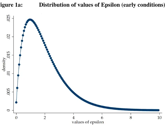
To provide a sense of the magnitude of these effects and some insight into the relations described above, we briefly discuss the results of a highly stylized numerical example. The main features of the exercise are as follows: (a) Individuals in the population are characterized by a latent variable εwith a Gamma distribution 𝑓(ε) with parameters 2 and 1 (with a mean and a variance equal to two). Whenever ε exceeds a threshold value (to be determined), the individual experiences poor early conditions and can potentially express excess mortality risks. (b) The mortality decline is defined so that the mortality rate at age y and t years after the onset of mortality decline is
µ(𝑦,𝑡) =𝑔(𝑡)∗ µ𝑠(𝑦,𝑡), (1)
where µ𝑠(𝑦,𝑡) is a standard mortality rate, and 𝑔(𝑡) is a (positive valued) function declining on t. Individuals who belong to group A experience mortality rates equal to
µ𝐴(𝑦,𝑡) =𝑔(𝑡)∗ µ𝑠(𝑦,𝑡)∗λ1 (2)
at all ages below 60, and equal to
µ𝐴(𝑦,𝑡) =𝑔(𝑡)∗ µ𝑠(𝑦,𝑡)∗λ2 (3)
at 60 and above with λ2 >λ1. Members of group B experience
µ(𝑦,𝑡) =𝑔(𝑡)∗ µ𝑠(𝑦,𝑡). (4)
(c) We set the values of λ2 𝑎𝑛𝑑λ1to be as small as 1.5 and as large as five. (d) We compute 100 cohort mortality “regimes” mimicking the mortality decline in the LAC region from 1941 to 2000, and then from 2000 to 2040 following the profile of UN mortality projections.
Figures 1a through 1c illustrate selected results of the calculations for a scenario in which the fraction of individuals experiencing early conditions is about
. 20 (ε>= 3),λ1 = 2 𝑎𝑛𝑑λ2 = 410F
11 . (5)
11 Other scenarios lead to similar conclusions. But, of course, more benign scenarios dilute the effects we seek
to highlight. For example, when the proportion of individuals who are exposed to early conditions is less than 5%, Barker effects are hardly visible and distinguishable, irrespective of values of λ1 and λ2 , from those that
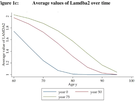
Figure 1a shows the initial distribution of ε. Figure 1b displays survival probabilities at the onset and at the end of the mortality decline (life expectancies of about 45 and 80, respectively) and for the members of group A in each case. Figure 1c displays the average values of λ2at age 60 throughout the decline. This figure shows the effects of the mortality decline on compositional changes across cohorts over the period of the decline. In year zero, the values of λ2are lower than 1.75 (the average value at time zero among those aged 60), irrespective of age. In years 50 and 75 (the two highest lines), the mean values of λ2 increase substantially, reflecting extra survival among individuals born with poor prospects; e.g., higher values of λ2.
Finally, Figure 1d displays the average mortality rates and the standard mortality rates (group B) at ages 65, 75, and 85 over the 100 years of observation. This is the ultimate outcome of the changes in composition induced by mortality decline. Thus, the average mortality (ages 65, 75, and 85) does not improve at the same rates as the baseline hazards rates do; instead, mortality does not improve at all or it may even increase, at least in some time periods.
Although this exercise is limited to only one out of many possible scenarios, the results are more general. Indeed, we can show that if, as assumed above, the early conditions are treated as a binary variable, a mortality decline resembling the one experienced in the LAC countries will produce results consistent with the hypothesis formulated above as long as the fraction in group A exceeds 0.15, and the values of λ1
and λ2 are larger than 1.5.12
12 It is important to highlight the simplifications that lead to these results. First, although we assumed Barker
Figure 1a: Distribution of values of Epsilon (early conditions)
Figure 1c: Average values of Lamdba2 over time
5. Empirical bounds for the effects of the early-late health
connection
Estimates from the generalized stable populations indicate that between 30% and 40% of the rate of increase in the population aged 60 and above between the years 2000 and 2020 in the LAC region is associated with the post-1940 mortality decline (Palloni et al. 2006). Thus, the rate of increase in the number of elderly in the region is, at least in part, the product of augmented survival among individuals who were exposed to or contracted infectious and parasitic illnesses, but who survived these diseases as a result of bolstered recovery rates. In the post-2000 period, an increasing fraction of the elderly will belong to birth cohorts whose members survived infectious and parasitic diseases that, prior to the mortality decline, would have killed them. To the extent that a non-trivial share of this mortality decline is dependent on the efficacy of medications, the fraction of adult individuals in a cohort who are likely to have experienced sub-optimal nutrition and frequent episodes of infections and parasitic diseases during childhood will increase over time. Furthermore, if the Barker effects are strong, the prevalence of adult chronic illnesses and the associated mortality risks will also increase.13 Under these conditions, life expectancy and healthy life expectancies at older ages could increase more slowly, or they could cease to increase altogether, even if the “background” mortality (i.e., mortality unrelated to early conditions) continues to decline. Below, we calculate the bounds for these effects, and show that under plausible conditions they can significantly decelerate the rate of decline of older mortality.
5.1 Estimation of the population exposed and excess mortality risk
We need to estimate two quantities. The first is the share of the population aged 60 and over who are more likely to be at risk of developing adult chronic diseases early in life. This population survived health regimes that combined poor nutritional status and high levels of exposure to infectious diseases with lower fatality rates. We call this the “exposed” population. The second is the Barker effect or the excess mortality among those who are at risk, or the exposed population. We use these two quantities to compute attributable mortality and the magnitude of the years of life expectancy losses.
Population exposed: the subpopulation aged 60+ at time t that is a direct result of the mortality decline that took place starting in 1930 is a function of the improvements in mortality, in both childhood (ages 0-4) and adulthood (ages 5-59). The magnitude of
13 If the association between early exposure to infection and late inflammation is negative, as McDade et al.
the mortality changes experienced in most low-income countries, particularly in LAC, is quite large, and an important share of it takes place between ages zero and five. Under a steady birth cohort size, the improvement experienced between 1950 and 1990 will, on average, represent extra growth of the population at age 60 of about 53 percent.14 This figure is an upper bound, since successive cohorts did not experience all at once the mortality change that took 30 to 40 years to unfold.
We can be more precise and partition the improvement into several components. Let B(t) stand for the size of a birth cohort in, say, 1950; let𝑆(1,𝑂) and 𝑆(1,𝑁) be the probabilities of surviving from birth to age five in the pre- and post-transitional mortality regimes, respectively; and let 𝑆(2,𝑂) and 𝑆(2,𝑁) be the conditional survivorship from age five up to age 60 exactly in the pre- and post-transitional mortality regimes, respectively. Finally,
𝑆(𝑂) =𝑆(1,𝑂)∗ 𝑆(2,𝑂) and 𝑆(𝑁) =𝑆(1,𝑁)∗ 𝑆(2,𝑁) (6) are the unconditional probabilities of surviving from birth to age 60 in the pre- and post-transitional mortality decline. The total (observed) population at age 60 at time t+60 is given by
𝑃𝑜 (𝑡+ 60, 60) = 𝐵(𝑡)∗ 𝑆(𝑁) = 𝐵(𝑡) ∗ 𝑆(1,𝑁) ∗ 𝑆(2,𝑁) (7) The total (counterfactual) population who would have reached age 60 under the pre-transitional mortality regime is
𝑃𝑐 (𝑡+ 60, 60) = 𝐵(𝑡)∗ 𝑆(𝑂) = 𝐵(𝑡) ∗ 𝑆 (1,𝑂)∗ 𝑆(2,𝑂) (8) The difference between Po and Pc which we denote by Δ, is the sum of the weighted
contribution of two components: one is equivalent to the contribution of changes in survival between ages zero and five and the other the equivalent of the contribution of changes in the conditional survivorship from age five up to age 60.15 The first component represents the growth of the population at age 60 that would have been observed if only early childhood mortality had changed and the survivors had been exposed to an adult pre-transitional mortality regime. The second component represents the growth of the population at age 60 that would have been observed if the mortality shift had only affected survivorship over age five, but survival between birth and age
14 This quantity was calculated assuming a change from a female life table in the West Coale-Demeny model
with a life expectancy equal to 40 to one with a life expectancy equal to 70.
15 The full expression is 𝛥 = 𝐵(𝑡) ∗(.5∗[(𝑆(1,𝑁)∗ 𝑆(2,𝑁) −𝑆(1,𝑂)∗ 𝑆(2,𝑁)) + (𝑆(1,𝑁)∗
five had followed the old mortality regime. The quantity Δ represents the population at age 60 added by the mortality decline in the interval (t, t+60). Alternatively, Δ is the population aged 60 in (t+60) who would not have been alive had it not been for the mortality improvements that took place between 1950 and 2010. The quantity Δ includes not only those who were saved because of changes in mortality between ages zero and five, but also those who survived because of mortality improvements at older ages. The quantity Δ can be calculated exactly by comparing the results of two population projections: one using the observed mortality schedules and one using the past (unchanged) mortality schedules.16
Δ is not a good measure of the size of the population exposed to the risk of expressing early-late health connections because it also includes a subpopulation who were saved due to mortality decline associated with improvements in the standard of living and public health. This segment of the population are less susceptible to express Barker effects, and we should exclude them from the population exposed. To estimate these two subpopulations composing Δ, we employ two procedures that can be used either jointly or separately. The simplest of these is to estimate the fraction of the mortality decline associated with improvements in income and living standards (as opposed to the diffusion of medical innovations and public health), and to partition Δ accordingly. The second is to use information on the relative contribution to the mortality decline of various causes of deaths. Since some causes of deaths are much more responsive to medical technologies than others (Palloni and Wyrick 1988; Preston 1976), we can use this knowledge to estimate the bounds for the fraction of the total population “saved” by the mortality decline who were more likely to have experienced poor early conditions. The first procedure (factor-specific) requires knowledge of the fraction of the total mortality decline due to medical innovations and improvements in the standard of living. The second procedure (cause-specific) is based on counterfactual projections by causes of death that result in estimates of the population “saved” associated with each cause-of-death-specific mortality decline. Finally, we could combine these two procedures and estimate cause-specific-factor-specific components. In what follows, we only use the first procedure.
The above identification of subpopulations is not sufficient, since we still need to assume that all of the individuals whose survival chances were ameliorated by medical technology are equally likely to express the effects of early conditions. This is too crude. By the same token, it would be too crude to assume that all those whose survival chances were augmented by improvements in standards of living are not at risk of expressing effects of early conditions. In the absence of additional information, we assume that in each case, there is a lower and an upper bound for the probability of expressing poor early conditions. As a lower bound, we use the average proportion of
low birth-weight infants born during the period 1960-1980 (0.10) The upper bound is the fraction of children who are stunted within the age interval one to 10 in a poor population (0.18 in INCAP, Guatemala). Admittedly these are rough bounds and introduce unavoidable uncertainty in our estimates.17 We now define the nature of the mortality excesses associated with the experience of early conditions.
Excess mortality risks or Barker effect: The second parameter required to estimate the desired bounds is the magnitude of excess mortality risks associated with exposure to early conditions. In principle, these excess risks are a function of the type of mechanism linking early conditions and adult morbid conditions: intrauterine deprivation could increase the risk of heart disease, which could in turn translate into excess mortality due to ischaemic heart disease. But an alternative mechanism, such as malnutrition during the first five years of life, may influence the likelihood of contracting type 2 diabetes, and may produce excess mortality due to kidney failure or circulatory impairments. The mortality risks are different in each case, and a precise estimation requires an assessment of the distribution of individuals according to their exposure to each of these distinct risks. Although this information is unavailable, we do have access to estimates of total excess mortality risks among those who experience some type of deprivation early in life. We assess the excess mortality risks associated with early deprivation by estimating logit models (with suitable controls) for the probability of dying at ages 60+ using data from multiple wave panel surveys of elderly people in three LAC countries. These models yield remarkably consistent estimates of excess mortality, with the relative risks contained within the 1.5-2.5 range.18
5.2 Computations
Following the rules established in 5.1 above, a birth cohort is first partitioned into two subpopulations. The first corresponds to the population who would have been observed irrespective of mortality decline. This represents a fraction 1-∆ (baseline) of the birth cohort. The second subpopulation can only be observed as a result of mortality decline, and represents a fraction ∆ (counterfactual) of the birth cohort. Each of these two
17 Even in a completely “Barkerian” environment, the lower and the upper bounds determined by the fraction
of low birth weight and the prevalence of malnutrition among children are likely to overestimate the true parameter, since not all low birth-weight infants or stunted children experience the same risks of developing adult chronic conditions. Conversely, some of those who are neither low birth-weight nor stunted could conceivably experience Barker effects.
18 The models to estimate the effects of exposure to early conditions on mortality are logistic models that
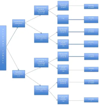
subpopulations is composed of a fraction λ who survived due to medical innovations; and the complementary share, 1-λ, who survived due to improvements in living standards. Finally, each of these four subpopulations is divided into a fraction who expressed early conditions, ϕ; and the complement, 1-ϕ, who did not. The total number of subpopulations thus created is eight, and for each cohort aged x at time t they will represent a fraction 𝑑(𝑥,𝑗,𝑡) of the total birth cohort. Thus, 𝑑(𝑥, 1,𝑗), the first subpopulation defined above, represents a fraction equal to
(1−∆)∗ λ∗ ϕ; 𝑑(𝑥, 2,𝑡), (9)
the second subpopulation defined above, represents a fraction equal to
(1−∆)∗ λ∗ (1−ϕ), (10)
and so on (see Figure 2). Each of these subpopulations is associated with mortality risks that are solely dependent on whether or not the members of the subpopulation express the effects of early conditions. If they do, they will experience a mortality excess equal to𝜇𝑜𝑒𝑥𝑝(β); if they do not, they will experience background mortality, 𝜇𝑜. The bottom of Figure 2 displays the eight components of a birth cohort and identifies the mortality levels that each of them experience. The terminal point of each branch in the figure is associated with the mortality risk characteristic of each subpopulation. The overall force of mortality at any age 60 and over and time t is calculated by averaging the mortality rate across all eight subpopulations:
5.3 Simplifications
To simplify the computations, we introduce several assumptions. First, the only quantity that must per force change over time is the fraction “saved,” since this quantity depends on population projections. All of the other quantities, particularly the distribution of the population by early conditions, are assumed to have been constant from 2000 onward. With one exception, this assumption does not interfere with our argument, and relaxing it will not affect the calculations in any significant way. The assumption will be unrealistic if the shift in mortality occurs simultaneously with, anticipates with a short lag, or even triggers a decline in fertility. This by itself is not sufficient to weaken the estimates. A violation of the assumption will damage the estimates if the fertility decline induced by the mortality changes produces better birth outcomes and/or promotes higher quality investments in children. In this case, we can no longer assume that the distribution by early conditions remains unchanged.
Second, the counterfactual projection sets all mortality rates between ages zero and 60, and not just infant and child mortality rates, to their 1950 levels. This means that we will include among those who could express early conditions at older ages a subgroup who survived the first five years of life, but who would have died before age 60 under the old mortality regime. Because these individuals are, by definition, less likely to have been exposed to adverse early conditions, we will exaggerate the effects of cohort changes. However, since mortality between ages five and 60 is low relative to child mortality, the bias will be small.19
Third, we will err on the conservative side and assume that the population size of the cohort component who would have survived in the absence of a mortality decline (component in the lower half of the graph), will not experience mortality excesses at all. This is a major simplification, and it can alter the bounds in significant ways, but always in the direction of downplaying the effects of cohort compositional changes.
5.4 Data and baseline estimates
We proceed in two stages. First, we project forward the population aged 50 and over starting in 1950 and ending in 2050. We do this using UN-projected life tables for 2010-2050 (United Nations 2002). We then repeat the projection, but while keeping mortality at the same levels as in 1950. This leads to estimates of differences between the observed and the counterfactual population for every year of the projection. Figure 3 displays the ratios of the observed to the counterfactual populations in the countries of interest for 2000-2050. The figure shows what we had expected: i.e., that the countries
with a more recent mortality decline have much smaller counterfactual populations (Guatemala). Indeed, the rank order of the curves in Figure 3 corresponds exactly to the ordering from an early to a late mortality decline.
Figure 3: Ratio of the total population aged 60+ from counterfactual projections (mortality at ages 0-59 kept at 1950 levels) to the conventional projected population
The second stage consists of calculating estimates of the excess mortality due to poor early conditions. The computations were carried out with data from three recent surveys of elderly people: the MHAS (Mexican Health and Aging Survey), the CRELES (Costa Rican Longevity and Health and Aging Study), and the PREHCO (Puerto Rican Elderly Health Study). The procedure consists of estimating logistic models for mortality over age 60 over an inter-wave period that varied between two years (MHAS) and six years (PREHCO). The model includes an indicator of exposure to poor early conditions, and controls for age, gender, education, and SES. We then use the estimated effects of the variable for early conditions as a measure of the Barker effect. In all cases, the coefficients were properly signed and were statistically significant. The relative risks were as small as 1.20 (CRELES) and as large as 1.9
0.40 0.50 0.60 0.70 0.80 0.90 1.00
2010 2015 2020 2025 2030 2035 2040 2045 2050
(PREHCO).20 Needless to say, these are not ideal estimates, but are coarse approximations because the identification of early conditions by older respondents has not been validated, and we know little about their correspondence with the early conditions that are of real significance (except perhaps for anthropometry that enables the identification of early malnutrition). Even if our indicators were accurate, the estimates from the logistic models could be subject to errors due to a misspecification of the model. It should be noted, however, that we used a sample of old-age survivors who underrepresent the population who experienced the worst conditions. Thus, the estimated effects will be downwardly biased.
5.5. Results
We now calculate the mortality rates above age 60 and the corresponding life expectancy at age 60 for several counterfactual scenarios. For each scenario we proceed as follows:21
a) We determine the counts of the “saved” and “not saved” populations by age. We call these S and NS.
b) We partition the saved population into a component who owe their survival to medical technology 𝑆 ∗λ, and another who owe their survival to socioeconomic conditions 𝑆 ∗(1−λ).
c) Each of the above populations is in turn divided into two subpopulations: one exposed to early conditions, 𝑆 ∗λ ∗ϕ1and 𝑆 ∗(1−λ) ∗ϕ2and another not exposed to early conditions, 𝑆 ∗ λ ∗(1−ϕ1) and 𝑆 ∗(1−λ)∗ �1−ϕ2�, where we allow for the possibility that those saved by forces other than medical conditions have a lower probability of experiencing early conditions (ϕ1>ϕ2).22 d) We calculate the mortality rates for each of the subpopulations created above. We
use as a baseline the UN mortality rates for 2000 and adopt the rates of decline assumed by the UN from 2000 through 2050. For each subpopulation exposed to early conditions, we increase the baseline mortality by the relative risk or mortality excess estimated before.23
20 We use an indicator of poor early conditions that is comparable across all three studies. The indicator pools
are based on a score that pools together (a) short knee height, (b) the respondent’s identification of poor health before age 15, and (c) self-reported poor SES before age 15.
21 Greek letters correspond to items in Figure 2.
22 Given our previous discussion, we use two alternative values for λ (0.40 and 0.60) and set ϕ
1 to be equal
0.38 and ϕ2 to be equal to 0.12.
23 The nature of the baseline mortality we choose does, of course, change the value of the quantities we
e) For each quinquennial period, we calculate the average mortality rates across all of the subpopulations identified above and the associated life expectancy at age 60.
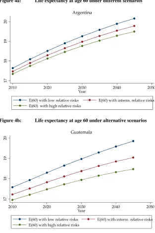
Figures 4a and 4b display the values of life expectancies at age 60 under three different scenarios for the two countries that produce extreme results, Argentina and Guatemala. At the beginning of the period under examination, there can be only small differences between alternative scenarios, since the fraction of the total projected population “saved” must be very small. When the influx of cohorts born after 1950 into age groups over 60 begins to grow, the different scenarios start diverging and yield different life expectancies. A mild scenario (with low values of λ, ϕ, and relative mortality risks among those exposed to adverse conditions of about 1.5) applied to Argentina produces differences on the order of 0.1 to 0.4 years of life expectancy at age 60. A harsher mortality regime among those exposed to deleterious conditions (relative risks on the order of 1.9) leads to larger differences, or about 0.66 years of life expectancy. These values are small because Argentina’s mortality decline began very early, some 20 to 30 years previously; and had somewhat different roots. As a consequence, the share of the population saved after 1950 is much smaller, and the exposure to excess adult mortality is minimized. On the other hand, in Guatemala, a country more typical among those that did not experience mortality declines until after 1950, the potential losses in life expectancy at age 60 are larger. A benevolent set of parameters produces differences of about 0.80 years. But when those exposed to adverse early conditions are subjected to a harsher mortality regime, the differences are as large as 1.5 years, or close to eight percent of the total life expectancy at age 60.
Overall, these are not massive differences, but neither are they trivial. Let us consider the following: during the period 2010-2050, Guatemala is projected to add 2.3 years of life expectancy at age 60; thus, the potential losses calculated here are about half of the total projected gains. In Argentina, the potential losses are, on average, one-sixth of the expected gains. By the same token, during the period 1980-2000, life expectancy at age 60 increased by about five years among the forerunners of the mortality decline (Palloni and Pinto 2011). Figures 4a and 4b reveal that as little as 8% and as much as 20% of this gain can be forfeited in a span of 50 years solely as a function of changes in cohort composition by exposure to early conditions.
Figure 4a: Life expectancy at age 60 under different scenarios
6. Conclusions
The estimates described above represent the bounds for the impact on future life expectancy in the LAC region of changes in the composition of cohorts according to their early experiences. These bounds, and their implications for future life expectancy, rest on two fundamental conditions. The first is that experiences with poor early conditions—from maternal health immediately before and during pregnancy, in utero growth and developmental impairments, malnutrition during the first five years of life, and adversity and exposure to infectious diseases early in childhood—all leave an imprint that could be expressed as higher risks of developing chronic conditions in adulthood and excess mortality risks. It must also be the case that, to the extent that these early-late health connections exist, they will not be offset by advances in medical knowledge or technology.
The second assumption is that the regime of mortality decline that a country experiences acts as a sorter, sifting through members of birth cohorts and enhancing survival to adulthood among those who, under conditions that prevailed in the past, would not have survived their first few years of life, or, if they did, would not have reached their 60th birthday. Furthermore, it must be the case that none of the mechanisms producing an early-late health connection are blunted by feedbacks embedded in the regime of mortality decline; for example, by strong synergisms between nutrition and susceptibility or resistance to infectious diseases.
If both conditions apply, then the massive mortality shifts that took place after 1950 could have lasting consequences and may constrain future gains in life expectancy at older ages. We used rough procedures and computed coarse bounds to assess how strong the tug of the past could be. Our results are somewhat speculative, but suggest that the impact of forces set in motion by the mortality decline could be strong enough to require substantial background mortality improvements to offset the legacy of past mortality regimes.
Because our estimates of excess mortality associated with early conditions are conservative, the bounds we compute are likely to be too small. There is far more uncertainty surrounding the estimates of the size of the population who could manifest Barker frailty. In this case, even our low bounds could exaggerate the final effects. These two sets of errors—one affecting the estimates of excess mortality among an exposed population and the other affecting the estimates of the size of this population— are of opposite signs, and will offset each other. The result could be that our overall bounds may be just about right. But this, of course, cannot be confirmed until we observe the actual mortality trajectory of the cohorts involved.
be, connected to early experiences, such as smoking and obesity. These trends represent separate threats, and their effects will also take a long time to dissipate. Naturally, the combination of these past lifestyle risks with the changing composition of cohorts by early exposures could slow down or stop altogether progress in life expectancy at older ages, at least in the short term.
7. Acknowledgements
References
Allen, A. (2007). The Controversial Story of Medicine’s Greatest Life Saver. New York: W.W. Norton & Company.
Arriaga, E.A. and Davis, K. (1969). The pattern of mortality change in Latin America. Demography 6(3): 223-242. doi:10.2307/2060393
Aschner, P. (2002). Diabetes trends in Latin America. Diabetes/Metabolism Research and Reviews 18(3): 27–31. doi:10.1002/dmrr.280
Barbi, E. and Vaupel, J.W. (2005). Comment on “Inflammatory Exposure and Historical Changes in Human Life-Spans”. Science 308(5729): 1743. doi:10.1126/science.1108707
Barcelo, A., Aedo, C., Rajpathk, S., and Robles, S. (2003). The cost of diabetes in Latin America and the Caribbean. Bulletin of the World Health Organization 81(1): 19-27.
Barker, D.J.P. (1998). Mothers, Babies and Health in Later Life. New York: Churchill Livingstone.
Ben-Shlomo, Y. and Smith, G.D. (1991). Deprivation in Infancy or in Adult Life: Which is More Important for Mortality Risk? The Lancet 337(8740): 530-534. doi:10.1016/0140-6736(91)91307-G
CELADE. (2007). Latin America and the Caribbean. Demographic Observatory No. 4: Mortality. Santiago de Chile: United Nations Publication.
Chackiel, J. (2004). La dinamica demografica en America Latina. Serie: Poblacion y Desarrollo, No. 52. Santiago de Chile: Publicación de las Naciones Unidas.
Cheung, S.L.K. and Robine, J.M. (2007). Increase in common longevity and the compression of mortality: the case of Japan. Population Studies: A Journal of Demography 61(1): 85-97. doi:10.1080/00324720601103833
Corrada, M.M., Brookmeyer, R., Paganini-Hill, A., Berlau, D., and Kawas, C.H. (2009). Dementia incidence continues to increase with age in the oldest old: The 90+ study. Annals of Neurology 67(1):114-121. doi:10.1080/ 00324720601103833
Crimmins, E.M., Preston, S.H., and Cohen, B.(eds.) (2011). Explaining Divergent Levels of Longevity in High-Income Countries. Washington, D.C.: National Academy Press.
Danese, A., Pariante, C.M., Caspi, A., Taylor, A., and Poulton, R. (2007). Childhood Maltreatment Predicts Adult Inflammation in a Life-Course Study. Proceedings of the National Academy of Sciences of the United States of America 104(4): 1319-1324. doi:10.1073/pnas.0610362104
Danesh J., Whincup, P., Walker, M., Lennon, L., Thomson, A., Appleby, P., Gallimore, J.R., and Pepys, M.B. (2000). Low grade inflammation and coronary heart disease: prospective study and updated meta-analyses. British Medical Journal 321(7255): 199-204. doi:10.1136/bmj.321.7255.199
Dowd, J.B. (2007). Early Childhood Origins of the Income/Health Gradient: the Role of Maternal Health Behaviors. Social Science & Medicine 65(6): 1202-1213. doi:10.1016/j.socscimed.2007.05.007
Elo, I.T. (1998). Childhood Conditions and Adult Health: Evidence from the Health and Retirement Study. University of Pennsylvania:Population Aging Research Center Working Papers (Working Paper Series No. 98-03).
Elo, I.T. and Preston, S.H. (1992). Effects of Early-Life Conditions on Adult Mortality: A Review. Population Index 58(2): 186-212. doi:10.2307/3644718
Ezra, S., Kuh, D. and Ben-Shlomo, Y. (eds.) (2004). A Life Course Approach to Chronic Disease Epidemiology. New York: Oxford University Press. doi:10.1093/acprof:oso/9780198578154.001.0001
Ezzati, M. and Lopez, A.D. (2003). Estimates of global mortality attributable to smoking in 2000. The Lancet 362(9387): 847-852. doi:10.1016/S0140-6736(03)14338-3
Finch, C.E. and Crimmins, E.M. (2004). Inflammatory Exposure and Historical Changes in Human Life-Spans. Science 305(5691): 1736-1739. doi:10.1126/ science.1092556
Fong, I.W. (2000). Emerging Relations between Infectious Diseases and Coronary Artery Disease and Atherosclerosis. Canadian Medical Association Journal 163(1): 49-56.
Gluckman, P.D. and Hanson, M.A. (eds.) (2006). Developmental Origins of Health and Disease Cambridge: Cambridge University Press. doi:10.1017/ CBO9780511544699
Hertzman, C. (1994). The Lifelong Impact of Childhood Experiences: A Population Health Perspective. Daedalus 123(4): 167-180.
Horiuchi, S. and Wilmoth, J. (1998). Deceleration in the age pattern of mortality at older ages. Demography 35(4): 391-412. doi:10.2307/3004009
Hossain, P., Kawar, B., and El Nahas, M. (2007). Obesity and Diabetes in the Developing World—A Growing Challenge. New England Journal of Medicine 356(3): 213-215. doi:10.1056/NEJMp068177
Kain, J., Vio, F., and Albala, C. (2003). Obesity trends and determinant factors in Latin America. Cadernos de Saude Pública 19(1): 77–86. doi:10.1590/S0102-311X2003000700009
Kannisto, V. (1994). Development of oldest-old mortality, 1950-1990: Evidence from 28 developed countries. Odense: Odense University Press.
Kannisto, V. (2001). Mode and dispersion of the length of life. Population: 13(1): 159-171.
Kannisto, V., Lauritsen, J., Thatcher, A.R., and Vaupel, J.W. (1994). Reductions in Mortality at Advanced Ages: Several Decades of Evidence from 27 Countries. Population and Development Review 20(4): 793-810. doi:10.2307/2137662
Langley-Evans, S.C. (ed.) (2004). Fetal Nutrition and Adult Disease: Programming of Chronic Disease through Fetal Exposure to Undernutrition. Wallingford, UK: CABI Publishing and The Nutrition Society. doi:10.1079/9780851998213.0000 Lobo, A., Launer, L.J., Fratiglioni, L., Andersen K., Di Carlo A., Breteler, M.M.B.,
Copeland, J.R.M., Dartigues, J.-F., Jagger, C., Martinez-Lage J., Soinnen, H., and Hofman A. (2000). Prevalence of dementia and major subtypes in Europe: A collaborative study of population-based cohorts. Neurology 54(11): 4-9.
Lundberg, O. (1991). Childhood Living Conditions, Health Status, and Social Mobility: a Contribution to the Health Selection Debate. European Sociological Review 7(2): 149-162.
McDade, T. W., Kuzawa, C., Rutherford, J., and Adair, L. (2010). Early Origins of Inflammation: Microbial exposures in infancy predict lower levels of C-reactive protein in adulthood. Proceedings of the Royal Society, Biological Sciences 277(1684): 1129-1137.
Oeppen, J. and Vaupel, J.W. (2002). Broken Limits to Life Expectancy. Science 296(5570): 1029-1031. doi:10.1126/science.1069675
Olshansky, S.J., Passaro, D.J., Hershow, R.C., Layden, J., Carnes, B.A., Brody, J., Hayflick, L., Butler, R.N., Allison, D.B., and Ludwig, D.S. (2005). A Potential Decline in Life Expectancy in the United States in the 21st Century. Obstetrical & Gynecological Survey 60(7): 450-452. doi:10.1097/01.ogx. 0000167407.83915.e7
Palloni, A. and Wyrick, R. (1981). Mortality Decline in Latin America: Changes in the Structure of Causes of Deaths, 1950-1975. Social Biology 28(3-4): 187-216. Palloni, A., McEniry, M., Wong R., and Pelaez, M. (2006). The tide to come: elderly
health in Latin America and the Caribbean. Journal of Aging and Health 18(2): 180-206. doi:10.1177/0898264305285664
Palloni, A., Novak, B., and Pinto, G. (2012). The enduring effects of smoking in Latin America. Paper presented at the Population Association of America, San Francisco, April 2012.
Palloni, A. and Pinto-Aguirre, G. (2011). Adult mortality in Latin America and the Caribbean. In Rogers, R.G. and Crimmins, E.M. (eds.) International Handbook of Adult Mortality, International Handbooks of Population 2. New York: Springer.
Peña, M. and Bacallao, J. (2004). Obesity among the Poor: An Emerging Problem in Latin America and the Caribbean. Obesity and Poverty. A New Public Health Challenge 1(1): 3–10
Preston, S.H. (1976). Mortality Patterns in National Populations: With Special Reference to Recorded Causes of Death. New York: Academic Press.
Preston, S.H. (1980). Causes and consequences of mortality declines in less developed countries during the Twentieth Century. In Easterlin, R.A. (ed.). Population and Economic Change in Developing Countries. Chicago: University of Chicago Press.
Preston, S.H, Hill, M.E. and Drevenstedt, G.L. (1998). Childhood conditions that predict survival to advanced ages among African Americans. Social Science and Medicine 47(9):1231-1246. doi:10.1016/S0277-9536(98)00180-4
Scrimshaw, N.S. (1997). Nutrition and Health from Womb to Tomb. Food and Nutrition Bulletin 18(1): 1-19.
Scrimshaw, N.S. and SanGiovanni, J.P. (1997). Synergism of nutrition, infection, and immunity: an overview. American Journal of Clinical Nutrition 66(2): 464-477. Smith, G.D. and Lynch, J. (2004). Life Course Approaches to Socioeconomic
Differentials in Health. In Kuh, D. and Ben-Shlomo, Y. (eds.). A Life Course Approach to Chronic Disease Epidemiology. Oxford: Oxford University Press.
Stern, A.M. and Markel, H. (2005). The history of vaccines and immunization: familiar patterns, new challenges. Health Affairs 24(3): 611-621. doi:10.1377/ hlthaff.24.3.611
Stolnitz, G.J (1965). Recent mortality trends in Latin America, Asia, and Africa. Population Studies 19(2): 117-138.
Thatcher, A.R., Cheung, S.L.K., Horiuchi, S., and Robine, J.-M. (2010). The compression of deaths above the mode. Demographic Research 22(17): 505-538. doi:10.4054/DemRes.2010.22.17
United Nations (ed.). (2002). World population prospects. New York: United Nations. Vaupel, J.W., Manton, K.G., and Stallard, E. (1979). The impact of heterogeneity in
individual frailty on the dynamics of mortality. Demography 16(3): 439-454. doi:10.2307/2061224
Vaupel, J.W. and Yashin, A.I. (1987). Repeated resuscitation: How lifesaving alters life tables. Demography 24(1): 123-135. doi:10.2307/2061512
White, K.M and Preston, S.H. (1996). How many Americans are Alive because of Twentieth-Century Improvements in Mortality? Population and Development Review 22(3): 415-429. doi:10.2307/2137714