Population and evolutionary adaptive dynamics of a stochastic predator-prey model

Commun. Math. Biol. Neurosci. 2016, 2016:12 ISSN: 2052-2541

POPULATION AND EVOLUTIONARY ADAPTIVE DYNAMICS OF A STOCHASTIC PREDATOR-PREY MODEL

TAO FENG1_{, XINZHU MENG}1,2,∗

1_{College of Mathematics and Systems Science, Shandong University of Science and Technology,} Qingdao 266590, PR China

2_{State Key Laboratory of Mining Disaster Prevention and Control Co-founded by Shandong Province and the} Ministry of Science and Technology, Shandong University of Science and Technology,

Qingdao 266590, PR China

Copyright c2016 Tao Feng and Xinzhu Meng. This is an open access article distributed under the Creative Commons Attribution License, which permits unrestricted use, distribution, and reproduction in any medium, provided the original work is properly cited.

Abstract. This paper intends to develop a theoretical framework for investigating the evolutionary adaptive dy-namics of a stochastic differential system. The key to the question is how to build an evolutionary fitness function. Firstly, we propose a stochastic predator-prey model with disease in the prey and discuss the asymptotic behavior around the positive equilibrium of its deterministic equation. Secondly, by using stochastic population dynamics and adaptive dynamics methods, we propose a fitness function based on stochastic impact and investigate the con-ditions for evolutionary branching and the evolution of pathogen strains in the infective prey. Our results show that (1) large stochastic impact can lead to rapidly stable evolution towards smaller toxicity of pathogen strains, which implies that stochastic disturbance is beneficial to epidemic control; (2) stochastic disturbance can go against evo-lutionary branching and promote evoevo-lutionary stability. Finally, we carry on the evoevo-lutionary analysis and make some numerical simulations to illustrate our main results. The developed methodologies could potentially be used to investigate the evolutionary adaptive dynamics of the stochastic differential systems.

Keywords:stochastic predator-prey model; evolution branching; stationary distribution; disease in the prey; pop-ulation dynamics.

2010 AMS Subject Classification:34K50, 92D15.

∗_{Corresponding author}

E-mail address: [email protected] Received May 3, 2016

1. Introduction

After the pioneering work of Hadeler and Freedman [1] on three species eco-epidemiological systems, namely, sound prey (susceptible), infected prey (infective) and predator have been studied extensively by researchers. The three species eco-epidemiological system describes a predator-prey model where the prey is infected, and the predator preys on only the infected prey since infected prey may be weaker or less active. There are so many references in this context, we have just cited here some of them (e.g. see, [2-8] and the references therein). The main works include Hopf bifurcation [2-3], the stability of equilibrium points [4-6], extinction and permanence [7], and so on.

Recently, the evolution of predator-prey community has received much attention from sci-entists (e.g. see, [9-13] and the references therein). The adaptive dynamics method provides a useful tool to investigate the long-term evolutionary outcomes of a small mutation in the traits expressing the phenotypes. A classical method of building the evolutionary fitness function is based on a globally asymptotically stable positive equilibrium point of the autonomous dif-ferential system (e.g. see, [9-12]). Moreover, many researchers are interested in the adaptive evolution based on nonequilibrium population dynamics. Meng et al. [13] have constructed an invasion fitness function, which involves the average growth rate and settles in a nonequilibrium attractor of non-autonomous differential system.

Therefore, according to a deterministic predator-prey system, this paper proposes a stochas-tic predator-prey evolutionary model with infected prey, to explore the influence of stochasstochas-tic disturbance on the evolution of toxicity of pathogen strains.

Our main goal of this paper is to build an evolutionary fitness function which is based on stochastic differential system and investigates the adaptive dynamics of the proposed model. To this end, the rest of the paper is organized as follows. In the next section, we first propose a stochastic predator-prey system with infected prey, then we study the global asymptotic behav-ior around the equilibrium of the deterministic predator-prey system. In Section 3, we build a fitness function to study the evolutionary dynamics of a single state. In the last section, we summarize our main results and focus our discussion on biological meaning.

2. Model and demographic properties

2.1. Population dynamics

We first consider a deterministic predator-prey system [2, 5], which reads 

     

     

dS

dt =rS(t)

1−S_K(t)−βS(t)I(t), dI

dt =βS(t)I(t)−cI(t)−pI(t)Y(t)−aI 2_(t),

dY

dt =k pI(t)Y(t)−dY(t),

(2.1)

whereS(t)andI(t), respectively, stand for the density of susceptible prey and infected prey at timet, Y(t)represents the population density of predator at time t. K represents the environ-mental maximum capacity, β is the infection rate from susceptible prey S(t)to infected prey

I(t),k(0≤k≤1)is the conversion rate from prey to a predator,ris the intrinsic growth rate of

S(t), pis the probability that infected prey is attacked by predator,ais the intraspecific compe-tition coefficient ofI(t), cis the diseased death rate ofI(t), d represents the natural death rate of predator.

Easy, if

R= k p d

r− cr

βK

β+ a

βK

system (2.1) has a positive equilibrium(S∗,I∗,Y∗)with

S∗= K(rk p−βd)

rk p , I

∗₌ d

k p, Y

∗₌ βK(rk p−βd)−rk pc−rda

rk p2 .

In the real world, biological populations are often disturbed by environmental interference. Therefore, it is important to investigate the effects of environmental noises on the properties of the systems. In this paper, we firstly study the following stochastic population dynamics system

      

     

dS=hrS(t)1−S_K(t)−βS(t)I(t) i

dt+σ1S(t)dB1(t),

dI=βS(t)I(t)−cI(t)−pI(t)Y(t)−aI2(t)dt+σ2I(t)dB2(t),

dY = [k pI(t)Y(t)−dY(t)]dt+σ3Y(t)dB3(t),

(2.2)

whereB_i(t)(i=1,2,3)is independent Brownian motions with intensityσ_i2(i=1,2,3).

Throughout this paper, let(Ω,F,{F}t≥0,P)be a complete probability space with a filtra-tion {Ft}t≥0 satisfying the usual conditions (i.e. it is increasing and right continuous while

F0 contains allP−null sets. FunctionBi(t)(i=1,2,3)is a Brownian motion defined on the complete probability space Ω. For an integrable function f on [0,+∞), we define hf(t)i= t−1R₀t f(s)ds.

2.2. Asymptotic behavior around the equilibriumE= (S∗,I∗,Y∗)of system (2.1)

In this subsection, we consider the asymptotic behavior around the equilibriumE= (S∗,I∗,Y∗)

of system (2.1).

X(t) is a temporally homogeneous Markov process in E_l, which is given by the stochastic differential equation

dX(t) =b(X)dt+

k

∑

m=1

σm(x)dBm(t),

whereE_l⊂Rl represents al-dimensional Euclidean space. The diffusion matrix ofX(t)is given by

Λ(x) = (ai,j(x)),ai,j(x) = k

∑

m=1

σ_mi(x)σ_mj(x).

(1) In the domain U and some of its neighbors, the minimum eigenvalue of the diffusion

matrix A(x)is nonezero.

(2) When x∈E_l\U , the mean timeτ at which a path starting from x to the set U is limited,

andsup x∈H

E_xτ<∞for every compact subset H⊂El.

Lemma 2.1.[22]When Assumption 2.1 holds, the Markov process X(t)has a stationary distri-bution µ(·)with density in El. Let f(x)be a function integrable with respect to the measure µ,

where x∈E_l, then for any Borel set B⊂E_l, we have

lim t→∞

P(t,x,B) =µ(B),

and

Px

lim T→∞

1

T Z T

0

f(x(t))dt = Z

El

f(x)µ(dx)

=1.

Theorem 2.1.Let(S(t),I(t),Y(t)be the solution of model (2.2). If R>1,σi>0,1≤i≤3and 0<δ<min{m1S∗2,m2I∗2,m3Y∗2}, then model (2.2) has a unique stationary distributionµand

it is ergodic. Here E = (S∗,I∗,Y∗)is the positive equilibrium of system (1),(S(0),I(0),Y(0)∈

R3₊ is the initial value,

η= 2K

r r−

r KS

∗₊ r

KI

∗₊1

k r KY

∗₊(r−2KrS

∗_−c−2aI∗₎2

2c +

(r−2_KrS∗−d)2

2d

!

,

ϖ=aη+aI∗+c 2−aS

∗₋a

kY

∗_,

m₁= rη

2K −σ

2

1,m2=ϖ−σ22,m3= 1

2k2 d−2σ

2 3

and

δ =σ₁2S∗2+σ₂2I∗2+ 1

k2σ 2 3Y∗

2

+(c+2aI

∗_+d)σ2 3Y∗

2k2_p +

η 2(σ

2

1S∗+σ22I∗+ 1

kσ

2 3Y∗).

Also we have

lim t→∞sup

1

tE Z t

0

m1(S(s)−S∗)2+m2(I(s)−I∗)2+m3(Y(s)−Y∗)2

ds≤δ.

Proof.Noting that(S∗,I∗,Y∗)is the positive equilibrium of model (2.1), one sees that

r

1−S

∗

K

Let us now define

V(S,I,Y) =η

S−S∗−S∗log S

S∗+I−I

∗_−I∗_log I

I∗+

1

k

Y−Y∗−Y∗log Y

Y∗

+1

2

S−S∗+I−I∗+1 k(Y−Y

∗₎

2

+ 1

k2

c+2aI∗+d p

Y−Y∗−Y∗log Y

Y∗

:=ηV1+V2+ 1

k2

c+2aI∗+d

p V3.

Applying Itˆo’s formula to stochastic differential system (2.2) yields

dV₁=

(S−S∗)

r

1− S

K

−βI

+S

∗_σ2 1 2

dt+σ1(S−S∗)dB1(t)

+

(I−I∗) [βS−c−aI−pY] +

I∗σ₂2 2

dt+σ2(I−I∗)dB2(t)

+1

k

(Y−Y∗) [k pI−d] +Y ∗

σ₃2

2 dt+σ3(Y−Y

∗_)dB

3(t)

:=LV1dt+σ1(S−S∗)dB1(t) +σ2(I−I∗)dB2(t) + 1

kσ3(Y−Y

∗_)dB

3(t),

where

LV₁=(S−S∗)

r

1− S

K

−βI

+S

∗

σ₁2

2 + (I−I

∗_{) [}

βS−c−aI−pY] +I

∗

σ₂2 2

+1

k

(Y−Y∗) (k pI−d) +Y ∗

σ₃2 2

=r(S−S∗)− r

K(S−S

∗₎2₋ r

K(S−S

∗_)S∗₋

β(S−S∗)(I−I∗)−β(S−S∗)I∗

+S

∗

σ₁2

2 −a(I−I

∗₎2_−a(I−I∗_)I∗₊

β(S−S∗)(I−I∗) +β(I−I∗)S∗

−c(I−I∗)−p(I−I∗)(Y−Y∗) +I ∗

σ₂2 2 −pY

∗_(I−I∗₎

+1

k

k p(Y−Y∗)(I−I∗) +k pI∗(Y−Y∗)−d(Y−Y∗) +Y ∗

σ₃2 2

=− r

K(S−S

∗₎2_−a(I−I∗₎2₊1 2

σ₁2S∗+σ₂2I∗+1

kσ

2 3Y∗

.

(2.3)

Let

dV₃=

(Y−Y∗)(k pI−d) +Y ∗_σ2

3 2

dt+ (Y−Y∗)σ3dB3(t)

then

LV₃= (Y−Y∗)(k pI−d) +Y ∗

σ₃2

2 =k p(Y−Y

∗_)(I−I∗_{) +}Y∗σ32 2 . Let

Z=S−S∗+I−I∗+1 k(Y−Y

∗_),

then

dZ=

rS− r

KS

2_−cI−aI2₋d

kY

dt+σ1SdB1(t) +σ2IdB2(t) + 1

kσ3Y dB3(t).

Easy,

dV₂=

S−S∗+I−I∗+1 k(Y−Y

∗ )

(

rS− r

KS

2_−cI−aI2₋d

kY

dt+σ1SdB1(t)

+σ2IdB2(t) + 1

kσ3Y dB3(t)

)

+1

2

σ₁2S2+σ₂2I2+ 1

k2σ 2 3Y2

dt

:=LV₂dt+

S−S∗+I−I∗+1 k(Y−Y

∗₎

σ1SdB1(t) +σ2IdB2(t) + 1

kσ3Y dB3(t)

,

where

LV₂=

S−S∗+I−I∗+1 k(Y−Y

∗_{) rS−} r

KS

2_−cI−aI2₋d

kY

+1

2

σ₁2S2+σ₂2I2+ 1

k2σ

2 3Y2

.

Since

rS− r

KS

2_−cI−aI2₋d

kY

=rS− r

K(S−S

∗₎2₊ r

KS

∗2₋2r

KSS

∗_{−cI−a(I−I}∗₎2_+aI∗2₋

2aII∗−d

kY

=− r

K(S−S

∗₎2₊

r−2r

KS

∗

S+ r KS

∗2_−cI−a

(I−I∗)2+aI∗2−2aII∗−d

kY

=− r

K(S−S

∗₎2₊

r−2r

KS

∗

(S−S∗) +

r− r

KS

∗_S∗_−c(I−I∗_)−cI∗

−a(I−I∗)2−aI∗2−2a(I−I∗)I∗−d

k(Y−Y

∗₎₋d

kY

∗

=− r

K(S−S

∗₎2₊

r−2r

KS

∗_(S−S∗_)−(c+

we have

LV₂=

S−S∗+I−I∗+1 k(Y−Y

∗₎

"

− r

K(S−S

∗₎2₊

r−2r

KS

∗_(S−S∗₎

−pI∗(Y−Y∗)−c+2aI∗

(I−I∗)−a(I−I∗)2

#

+1

2

σ₁2S2+σ₂2I2+ 1

k2σ 2 3Y2

=− r

K

S+I+1 kY

(S−S∗)2+

r− r

KS

∗₊ r

KI

∗₊1

k r KY

∗_(S−S∗₎2

−a

S+I+1 kY

(I−I∗)2+aS∗−aI∗+a kY

∗_−c(I−I∗₎2

+

r−2r

KS

∗_−c−2aI∗

(S−S∗)(I−I∗)

+1

k

r−2r

KS

∗_−d

(S−S∗)(Y−Y∗)−1

k(c+2aI

∗_{+d) (I−I}∗_)(Y−Y∗₎

− d

k2(Y−Y

∗₎2₊1 2

σ₁2S2+σ₂2(x)I2+ 1

k2σ

2 3Y2

≤

r− r

KS

∗₊ r

KI

∗₊1

k r KY

∗

(S−S∗)2+

aS∗−aI∗+a kY

∗_−c(I−I∗₎2

+

r−2r

KS

∗_−c−2aI∗

(S−S∗)(I−I∗) +1

2

σ₁2S2+σ₂2I2+ 1

k2σ 2 3Y2

+1

k

r−2r

KS

∗_−d(S−S∗_)(Y−Y∗₎₋1

k(c+2aI

∗_{+d) (I−I}∗_)(Y−Y∗₎

− d

k2(Y−Y

∗₎2_.

(2.4)

By the Cauchy inequality, it is easy to show that

r−2r

KS

∗_−c−

2aI∗

(S−S∗)(I−I∗)≤ c

2(I−I

∗

)2+(r−

2r KS

∗_−c−2aI∗₎2

2c (S−S

∗ )2 and 1 k

r−2r

KS

∗_−d(S−S∗_)(Y−Y∗_)≤ d

2k2(Y−Y

∗₎2₊(r− 2r KS

∗_−d)2 2d (S−S

We can show from (2.4) that

LV₂≤ r− r

KS

∗₊ r

KI

∗₊1

k r KY

∗₊(r−2KrS

∗_−c−2aI∗₎2

2c +

(r−2r KS

∗_−d)2

2d +σ

2 1

!

(S−S∗)2

+aS∗−aI∗+a kY

∗₋c

2+σ 2 2

(I−I∗)2− 1

2k2(d−2σ

2

3)(Y−Y∗)2

−1

k(c+2aI

∗

+d) (I−I∗)(Y−Y∗) +σ₁2S∗2+σ₂2(x)I∗2+ 1

k2σ 2 3Y∗

2 .

(2.5)

Easy, we have

LV₄=LV₂+c+2aI

∗_+d

k2p LV3

≤ r− r

KS

∗₊ r

KI

∗₊1

k r

KY

∗₊(r−2KrS

∗_−c−2aI∗₎2

2c +

(r−2_KrS∗−d)2

2d +σ

2 1

!

(S−S∗)2

+

aS∗−aI∗+a kY

∗₋c

2+σ 2 2

(I−I∗)2− 1

2k2(d−2σ 2

3)(Y−Y∗)2

+σ₁2S∗2+σ₂2(x)I∗2+ 1

k2σ

2 3Y∗

2

+(c+2aI

∗_+d)

σ₃2Y∗ 2k2p .

(2.6)

Consequently, from (2.3) and (2.6), one has

LV =ηLV1+LV4

≤ −rη

2K−σ

2 1

(S−S∗)2− ϖ−σ₂2(I−I∗)2− 1

2k2(d−2σ

2

3)(Y−Y∗)2

+σ₁2S∗2+σ₂2I∗2+ 1

k2σ 2 3Y∗

2

+(c+2aI

∗_+d)σ2 3Y∗

2k2_p +

η 2(σ

2

1S∗+σ22I∗+ 1

kσ

2 3Y∗)

=−m₁(S−S∗)2−m₂(I−I∗)2−m₃(Y−Y∗)2+δ.

(2.7)

For anyδ <min{m1S∗,m2I∗,m3Y∗}, the ellipsoid

−m₁(S−S∗)2−m₂(I−I∗)2−m₃(Y−Y∗)2+δ =0

lies entirely inR3₊. LetU to be any neighborhood of the ellipsoid with ¯U ⊆E₃=R3₊, thus for anyx∈U\E_l,LV ≤ −M(Mis a positive constant). Therefore, condition(2)in Assumption 2.1 is satisfied. Moreover, there exists aG=min{σ₁2x₁2,σ₂2x2₂,σ₃2x2₃,(x1,x2,x3)∈U}>0 such that

3

∑

i,j=1 3

∑

k=1

a_ik(x)a_jk(x)

!

for allx∈U¯,ξ ∈R3, which means condition(1)in Assumption 2.1 is satisfied. Therefore, the stochastic model (2.2) has a unique stationary distributionµ(·), it also has the ergodic property. Since

dV =LV dt+η

(S−S∗)σ1dB1(t) + (I−I∗)σ2dB2(t) + 1

k(Y−Y

∗₎

σ3dB3(t)

+

S−S∗+I−I∗+1 k(Y−Y

∗₎

σ1SdB1(t) +σ2IdB2(t) + 1

kσ3Y dB3(t)

+c+2aI

∗_+d

k2_p σ3(Y−Y

∗_)dB

3(t).

(2.8)

Integrating system (2.8) from 0 tot and taking the expectation on both sides yields

EV(t)−EV(0)≤ −m1E

Z t

0

(S(s)−S∗)2ds−m2E

Z t

0

(I(s)−I∗)2ds

−m₃E Z t

0

(Y(s)−Y∗)2ds+δt.

(2.9)

Dividing both sides of (2.9) bytand lett→+∞yields

lim t→∞

EV(t)−EV(0) t

≤ −1

t

m1E

Z t

0

(S(s)−S∗)2ds+m2E

Z t

0

(I(s)−I∗)2ds+m3E

Z t

0

(Y(s)−Y∗)2

ds+δ.

Easy,

lim t→∞sup

1

tE Z t

0

m₁(S(s)−S∗)2+m₂(I(s)−I∗)2+m₃(Y(s)−Y∗)2ds≤δ. (2.10)

This completes the proof.

Theorem 2.2. Assume that the conditions in Theorem 2.1 are met. Let (S(t),I(t),Y(t)) be a solution of model (2.2) with initial value(S(0),I(0),Y(0))∈R3₊. If

r> σ 2 1 2

and

k p

β(d+σ 2 3 2 )



r− σ₁2

2 −

r Kβ





a(d+σ22 2)

k p +c+

σ₂2 2



 

then the solution(S(t),I(t),Y(t))of model(2.2)satisfies                  P lim t→∞

1

t Z t

0

S(s)ds= Z

R3+

z1µ(dz1,dz2,dz3) =Se∗

=1, P

lim t→∞

1

t Z t

0

I(s)ds= Z

R3+

z₂µ(dz1,dz2,dz3) =eI∗

=1, P

lim t→∞

1

t Z t

0

Y(s)ds= Z

R3₊

z₃µ(dz1,dz2,dz3) =Ye∗

=1,

(2.11)

where                              e

S∗=K r



 r−

σ₁2 2 −

β

d+σ

2 3 2 k p   , e

I∗= d+

σ₃2

2

k p ,

e

Y∗= 1 p    Kβ r   r−

σ₁2 2 −

β

d+σ32 2 k p   −

a(d+σ

2 3 2 )

k p −c−

σ₂2 2



 .

Proof.By the definition of ergodic property, for anyw(wis a positive constant), one has lim

t→∞

1

t Z t

0

(S2(s)∧w)ds= Z

R3+

(z2₁∧w)µ(dz1,dz2,dz3)a.s. (2.12)

Using the dominated convergence theorem and equation (2.12), one can see that

E

" lim t→∞

1

t Z t

0

(S2(s)∧w)ds

#

=lim

t→∞

1

t Z t

0

E S2(s)∧w

!

ds<∞, (2.13)

Easy,

Z

R3+

(z2₁∧w)µ(dz1,dz2,dz3)<∞.

Letw→∞, one has

Z

R3+

z2₁µ(dz1,dz2,dz3)<∞.

In other words,S2is integrable with respect to the measureµ. By using the property of ergod-icity, one sees that

lim t→∞

1

t Z t

0

S(s)ds= Z

R3+

z₁µ(dz1,dz2,dz3)a.s. (2.14) Similarly, one can derive that

lim t→∞

1

t Z t

0

I(s)ds= Z

R3₊

and

lim t→∞

1

t Z t

0

Y(s)ds= Z

R3+

z3µ(dz1,dz2,dz3)a.s.

An application of Itˆo’s formula implies

dlogS=

r−1

2σ 2 1−

r

KS−βI

dt+σ1dB1(t),

Integrating the above equation from 0 tot yields logS(t)−logS(0) =

r−1

2σ 2 1

t− r

K Z t

0

S(s)ds−β

Z t

0

I(s)ds+σ1B1(t).

Dividing both sides of the above equation byt and lett →+∞, we have

lim t→∞

logS(t)

t =r−

1 2σ

2 1−

r

K Z

R3

+

z₁µ(dz1,dz2,dz3)−β

Z

R3

+

z₂µ(dz1,dz2,dz3):=ρ1. Ifρ1>0, there exists aT =T(ω)for anyt>T one has

logS(t)> ρ1

2 t. Then

lim t→∞

1

t Z t

0

S(s)ds→∞,

which is in contradiction with equation (2.14).

Ifρ1<0, there exists aT =T(ω)fort>T one gets that lim

t→∞

1

t Z t

0

S(s)d<0,

which is in contradiction with equation (2.14). Therefore

lim t→∞

logS(t)

t =0.

Similarly, one can derive that lim t→∞

logI(t)

t =0,tlim→∞

logY(t)

t =0.

So we have 

     

     

r−σ12 2 −

r K

R

R3+z1µ(dz1,dz2,dz3)−β

R

R3+z2µ(dz1,dz2,dz3) =0,

−c−σ22 2 +β

R

R3₊z1µ(dz1,dz2,dz3)−a

R

R3₊z2µ(dz1,dz2,dz3)−p

R

R3₊z3µ(dz1,dz2,dz3) =0,

−d−σ32 2 +k p

R

Moreover, there exists a positive solution(Se∗,eI∗,Ye∗)of equation             

r−σ12 2 −

r

KS−βI=0,

−c−σ22

2 +βS−aI−pY =0,

−d−σ32

2 +k pI=0,

(2.15)

ifr> σ 2 1 2 and

k p

β(d+σ 2 3 2 )



r− σ₁2

2 −

r

Kβ 



a(d+σ22 2 )

k p +c+

σ₂2 2



 

>1 are fulfilled. The above discussion gives

                 P lim t→∞

1

t Z t

0

S(s)ds= Z

R3+

z₁µ(dz1,dz2,dz3) =Se∗

=1, P

lim t→∞

1

t Z t

0

I(s)ds= Z

R3+

z2µ(dz1,dz2,dz3) =eI∗

=1, P

lim t→∞

1

t Z t

0

Y(s)ds= Z

R3₊

z₃µ(dz1,dz2,dz3) =Ye∗

=1.

(2.16)

This completes the proof.

3. Evolutionary adaptive dynamics

3.1. The model

When the resident population(the infected prey with trait x) was invaded by a rare mutant prey population with a markedly different traity, the predator-prey system (2.2) becomes

                            

dS=S(t)

r

1−S(t)

K

−β(x)I(t)−β(y)Imut(t)

dt+σ1S(t)dB1(t),

dI=I(t) [β(x)S(t)−c(x)−p(x)Y(t)−a(x,x)I(t)−a(x,y)Imut]dt+σ2(x)I(t)dB2(t),

dI_mut=I_mut(t) [β(y)S(t)−c(y)−p(y)Y(t)−a(y,y)Imut(t)−a(y,x)I(t)]dt

+σ2(y)Imut(t)dB2(t),

dY =Y(t)k p(x)I(t) +k0p(y)Imut(t)−d

dt+σ3Y(t)dB3(t),

(3.1)

predator at timet. β(x)andβ(y)stand for the infection rates from susceptibleS(t)to infected

I(t) with trait x and infectedI_mut(t) with trait y, respectively. c(x) and c(y) are the diseased death rates ofI(t)andImut(t), respectively. p(x)and p(y)represent the attack rates on infected preyI(t)and infected preyI_mut(t), respectively. The competition coefficienta(x,y)denotes the influence of traitxon traity, a(x,x)anda(y,y)are the intraspecific competition coefficients of

I(t)andI_mut(t), respectively.B_i(t)(i=1,2,3)are independent Brownian motions with intensity σ_i2(i=1,2,3),Krepresents the environmental maximum capacity,ris the intrinsic growth rate of S(t), d represents the natural death rate of predator. k and k0 (0≤k,k0≤1) stand for the conversion rates fromI(t)toY(t)and fromImut(t)toY(t), respectively.

Generally speaking, the more severe the disease is, the weaker the population’s ability to resist disturbance is. That is to say, the more severe the disease is, the more the dead diseased prey is. Therefore, we choose the following interference intensity function:

σ2(x) =v h

1−(1+0.2δx)exp(−0.2δx) i

, (3.2)

whereδ is a coefficient that is positively correlated with the intensity of stochastic perturbation,

v>0 is a constant. See Fig. 1.

0 5 10 15 20

0 0.2 0.4 0.6 0.8 1

Trait value x

σ2

(x)

δ=1

δ=2

δ=5

FIG. 1. Convex-concave shape of the intensity of noisesσ2(xi) as given by system

(3.2)(v=1).

The greater pathogenic toxicity of the virus in infected prey implies the greater infection rate, diseased death rate and predation rate. Therefore, in system (3.1), we choose the following infection rate function, diseased death rate function, attack rate function:

wherel,e₁,e₂are positive constants.

It is widely accepted that prey with serious disease is at a disadvantage to survive when competes with prey who has light disease. Therefore, the competition coefficienta(xi,xj)which denotes the influence of traitx_jon traitx_iis an increasing function, which is given by

a(x_i,x_j) = f

1− 1

1+mexp(w(x_i−x_j))

, (3.3)

where f,m,ware positive constants. See Fig. 2.

−50 0 5

0.5 1 1.5 2

x

i−xj

a(x

i

,x j

)

m=0.5 m=1 m=2

FIG. 2. Concave-convex shape ofa(xi,xj)as given by (3.3)(m=0.5; 1; 2;f =2;w=1.2).

LettingImut=0 and using the well-known Itˆo’s formula in the third equation of model (3.1), we get

dImut

I_mut =dlnImut=

h

β(y)S(t)−c(y)−p(y)Y(t)−a(y,x)I(t)−σ 2 2(y)

2 i

dt+σ2(y)dB2(t).

Let

F(x,y) =hβ(y)S(t)−c(y)−p(y)Y(t)−a(y,x)I(t)−σ 2 2(y)

2 i

dt+σ2(y)dB2(t). (3.4) Integrating both sides of equation (3.4) from 0 tot leads to

Z t

0

F(x,y)dt =β(y)

Z t

0

S(s)ds−

Z t

0

c(y)ds−p(y) Z t

0

Y(s)ds−a(y,x) Z t

0

I(s)ds−

Z t

0

σ₂2(y) 2 ds

+σ2(y) B2(t)−B2(0)

.

(3.5)

Dividing both sides of equation (3.5) byt yields

hF(x,y)i=β(y)hS(t)i −c(y)−p(y)hY(t)i −a(y,x)hI(t)i −σ 2 2(y)

2 +

σ2(y) B2(t)−B2(0)

Lettingt→∞, using limt→∞t−1B(t) =0 and limt→∞t−1B(0) =0, we see that

f(x,y)≡ lim t→∞h

F(x,y)i=β(y)Se∗−c(y)−p(y)Ye∗−a(y,x)eI∗− σ₂2(y)

2 , a.s. (3.6) Note that f(x,y)is the long-term average exponential growth rate of the mutant population. Hence, if f(x,y)is positive, then the mutant prey can invade, otherwise the resident prey can not be invaded and the mutant prey will die out. So f(x,y)is the fitness function[23]. Then we can obtain a local fitness gradientD(x)which determines the direction of evolution, andD(x)

is given by

D(x) =∂f(x,y)

∂y

y=x

=Kβ 0_(x)

r



 r−

σ₁2 2 −

β(x)

d+σ

2 3 2

k p(x)



 −c

0

(x)−a0(x,x)d+

σ₃2

2

k p(x) − p0(x)

p(x)

×



 

Kβ(x)

r



 r−

σ₁2 2 −

β(x)

d+σ

2 3 2

k p(x)



 −

a(x,x)(d+σ32 2 )

k p(x) −c(x)−

σ₂2(x) 2



 

−σ2(x)σ20(x).

(3.7)

IfD(x)>0, the mutant infectious prey with traitywhich is obviously bigger thanxcan invade and replace the resident infectious prey population, otherwise if the fitness gradientD(x)<0, the resident infectious prey population can be invaded and took over by the mutant infectious prey with traitywhich is obviously smaller thanx. Thus, we know that the direction of evolution is determined byD(x). Since mutations are random and sufficiently small, so the evolutionary dynamics of traitxcan expressed as [9]

dx

dt =

1 2µ σ

2 g

I(x)∗D(x), (3.8)

whereD(x)is the fitness gradient in equation (3.7),Ig(x)

∗

WhenD(x∗) =0, the trait x∗is called an evolutionary singular strategy. At the evolutionary singular strategy pointx∗, whether the evolution continues depends on its evolutionary stability and convergence stability. In the neighborhood of the evolutionary singular strategyx∗, if the resident population with strategyxwas invaded by the nearby mutant strategyy, thenx∗is called the convergence stable strategy.

According to (3.7), we know that in the vicinity ofx∗, ifx<x∗, thenD(x)>0, otherwise if

x>x∗, thenD(x)>0. Therefore, the condition for convergence stable is as follows

dD(x) dx

x=x∗

=− Kβ

0_(x∗₎

rk2_p2_(x∗₎

"

β0(x∗)

d+σ

2 3 2

k p(x∗)−β(x∗)

d+σ

2 3 2

k p0(x∗)

#

−p

00_(x∗_)p(x∗_)−p02_(x∗₎

p2_(x∗₎

"

Kβ(x∗)

r

r−σ

2 1 2 −

β(x∗)

d+σ32 2

k p(x∗)

−a(x

∗_,x∗_)(d+σ₃2

2)

k p(x∗) −c(x

∗₎₋σ2(x∗)2

2 #

−c00(x∗)−a00(x∗,x∗)d+

σ₃2

2

k p(x∗)

+a0(x∗,x∗) d+

σ₃2

2

k p2_(x∗₎−

p0(x∗) p(x∗)

"

Kβ0(x∗) r

r−σ

2 1 2 −

β(x∗)

d+σ

2 3 2

k p(x∗)

−

Kβ(x∗)

d+σ32 2

rk p2(x∗)

β0(x∗)p(x∗)−β(x∗)p0(x∗)

−

d+σ

2 3 2

k p2_(x∗₎

a0(x∗,x∗)p(x∗)−a(x∗,x∗)p0(x∗)−c0(x∗)−σ2(x∗)σ₂0(x∗) #

−σ₂02(x∗)−σ2(x∗)σ200(x∗) +

Kβ00(x∗)

r

"

r−σ

2 1 2 −

β(x∗)

d+σ32 2

k p(x∗)

#

<0.

(3.9)

The singular strategyx∗is evolutionary stable (i.e. ESS) if it satisfies

∂f2(x,y) ∂y

y=x=x∗

=Kβ 00_(x∗₎

r

"

r−σ

2 1 2 −

β(x∗)

d+σ

2 3 2

k p(x∗)

#

−c00(x∗)−a00(x∗,x∗)d+

σ₃2

2

k p(x∗)

−p

00_(x∗₎

p(x∗)

hK_β(x∗)

r

r−σ

2 1 2 −

β(x∗)

d+σ32 2

k p(x∗)

−a(x

∗_,x∗_)(d+σ₃2

2 )

k p(x∗)

−c(x∗)−σ2(x

∗₎2 2

i

−σ₂02(x∗)−σ2(x∗)σ₂00(x∗)<0.

The singular strategyx∗is a continuously stable strategy (i.e. CSS) if it is both convergence stable and evolutionary stable, which will bring the endpoint of the evolution. If the evolu-tionary singular pointx∗satisfies convergence stable but lacks evolutionary stable, it will brings evolutionary branching. In other words, the single population will become two different species. Otherwise, if the evolutionary singular strategyx∗is both convergence stable and evolutionary stable, the evolution will stop.

Proposition 3.1. If the singularity x∗of(3.8)satisfies inequalities(3.9)and(3.10), the evolu-tionary singular point x∗ is a continuously stable strategy (CSS); If the singularity x∗ of(3.8) satisfies (3.9) but does not satisfy (3.10), the evolutionary singular point x∗ is a branching point.

C

A +

+ —

—

—

0 1 2 3 4 5

0 1 2 3 4 5

x

y

HaL

B —

—

+ +

8.0 8.5 9.0 9.5 10.0 10.5 11.0 8.0

8.5 9.0 9.5 10.0 10.5 11.0

x

y

HbL

FIG. 3. Pairwise invasibility plots. The dashed areas marked with ‘+’ indicate that the fitness function f(x,y)>0, in contrast, the areas marked with ‘−’ say

f(x,y)<0. A is an evolutionary stable point, B is a branching point, C is a repeller. (a) Multisingular strategies whenδ =5; (b) The singular strategy is an evolutionary branching point whenδ =0.4;

is convergence stable but evolutionarily stable. Thusx∗is an evolutionary branching point, and all nearby mutant population can invade.

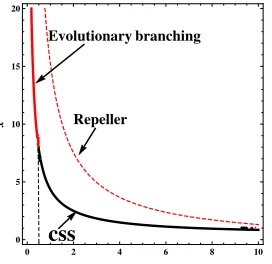
Repeller

Evolutionary branching

css

0 2 4 6 8 10

0 5 10 15 20

∆

x

FIG. 4. Bifurcation diagram for evolutionary singular strategy xand the intensity of

noiseδ. Red solid line represents unstable singular strategyx, black solid line represents

the CSS, and read dashed line represents the repeller. The parameter values are K=

1,k=0.1,d=0.1,r=0.1,σ1=0.1,σ3=0.2,v=1,m=2,w=1.2,f=1,l=0.5,e1=

0.05,e2=0.05.

x*

9.0 9.2 9.4 9.6 9.8 10.0

-0.004 -0.002 0.000 0.002 0.004

y

f

H

y

,x

L

HaL

x*

0 1 2 3 4

-5

-4

-3

-2

-1

0 1

y

f

H

y

,x

L

HbL

FIG. 5. Fitness landscape at the singular x∗. (a) δ =0.4; (b) δ =5; Other parameter values:K=1,k=0.1,d=0.1,r=0.1,σ1=0.1,σ3=0.2,v=1,m= 2,w=1.2,f =1,l=0.5,e₁=0.05,e₂=0.05.

the singular strategy will be changed. That is to say, noise with small intensity can lead to the evolutionary branching, in contrast, noise with large intensity may cause a continuous stability strategy (CSS). In Fig.5 (a), we chooseδ =0.4, it is easy to see that f(y,x)near strategyx∗is positive and convex, thus the strategy can experience evolutionary branching. In Fig.5(b), we chooseδ =5, we can see that f(y,x)near strategyx∗is negative and concave, thus the strategy can not experience evolutionary branching.

4. Discussion

This paper considers a stochastic predator-prey model with disease in the prey under white noise disturbances and this paper shows that the stochastic model has a unique stationary distri-bution with ergodic property. Furthermore, we investigate asymptotic behavior of the stochastic system around the endemic equilibrium of the deterministic model and we explored the evo-lution of pathogen virulence of diseased prey with phenotype traitx. By modeling population dynamics under these conditions, we gain the fitness function, then we give the conditions under which the resident diseased prey population experienced evolutionary branching. The biological significance of the results shows that an increase in the intensity of noise will cause the decrease in the singular strategy x. In addition, noise with small intensity can lead to the evolutionary branching, in contrast, noise with large intensity may cause a continuous stability strategy (CSS), which implies that the white noise stochastic disturbance is advantage for the control of the epidemic disease.

This paper intends to develop a theoretical framework for investigating the evolutionary adap-tive dynamics of a stochastic differential system. We apply our theoretical method to understand the evolutionary dynamics under stochastic differential equations. As a consequence, this pa-per proposes a new theoretical method for evolutionary adaptive dynamics based on stochastic differential equations. A promising extension of this work is to consider the environment with disturbance of L´evy jumps or Markov process.

Conflict of Interests

Acknowledgements

This work is supported by the National Natural Science Foundation of China (11371230, 11501331), the SDUST Research Fund (2014TDJH102), Shandong Provincial Natural Science Foundation, China (ZR2015AQ001, BS2015SF002), Joint Innovative Center for Safe And Effective Mining Technology and Equipment of Coal Resources, Shandong Province, a Project of Shandong Province Higher Educational Science and Technology Program of China (J13LI05).

REFERENCES

[1] K.P. Hadeler, H.I. Freedman, Predator-prey populations with parasitic infection, J. Math. Biol. 27 (1989), 609-631.

[2] J. Chattopadhyay, O. Arino, A predator-prey model with disease in the prey, Nonlinear. Anal. 36 (1999), 747-766.

[3] Y.N. Xiao, L.S. Chen, Modeling and analysis of a predator-prey model with disease in the prey, Math. Biosci. 171 (2001), 59-82.

[4] B. Mukhopadhyay, R. Bhattacharyya, Role of predator switching in an eco-epidemiological model with dis-ease in the prey, Ecol. Model. 220 (2009), 931-939.

[5] Y.N. Xiao, L.S. Chen, Analysis of a Three Species Eco-Epidemiological Model, J. Math. Anal. Appl. 258 (2001), 733-754.

[6] B.W. Kooi, G.A.V. Voorn, K.P. Das, Stabilization and complex dynamics in a predator-prey model with predator suffering from an infectious disease, Ecol. Complex. 8 (2011), 113-122.

[7] H.W. Hethcote, W.D. Wang, L.T. Han, Z.E. Ma, A predator-prey model with infected prey, Theor. Popul. Biol. 66 (2004), 259-268.

[8] L.T. Han, Z.E. Ma, Four Predator Prey Models with Infectious Diseases, Math. Comput. Model. 34 (2001), 849-858.

[9] U. Dieckmann, P. Marrowb, R. Law, Evolutionary cycling in predator-prey interactions: population dynamics and the red queen, J. Theor. Biol. 176 (1995), 91-102.

[10] J. Zu, M. Mimura, Y. Takeuchi, Adaptive evolution of foraging-related traits in a predator-prey community, J. Theor. Biol. 268 (2011), 14-29.

[11] J. Zu, J.L. Wang, Adaptive evolution of attack ability promotes the evolutionary branching of predator species, Theor. Popul. Biol. 89 (2013), 12-23.

[13] X.Z. Meng, R. Liu, T.H. Zhang, Adaptive dynamics for a non-autonomous Lotka-Volterra model with size-selective disturbance, Nonlinear. Anal. 16 (2014), 202-213.

[14] M. Liu, H. Qiu, K. Wang, A remark on a stochastic predator-prey system with time delays, Appl. Math. Lett. 26 (2013), 318-323.

[15] Q. M. Zhang, D.Q. Jiang, Z.W. Liu, D. O’Regan, The long time behavior of a predator-prey model with disease in the prey by stochastic perturbation, Appl. Math. Comput. 245 (2014), 305-320.

[16] C.Y. Ji, D.Q. Jiang, N.Z. Shi, Analysis of a predator-prey model with modified Leslie-Gower and Holling-type II schemes with stochastic perturbation, J. Math. Anal. Appl. 359 (2009), 482-498.

[17] J.L. Liu, K. Wang, Asymptotic properties of a stochastic predator-prey system with Holling II functional response, Commun. Nonlinear. Sci. 16 (2011), 4037-4048.

[18] M. Liu, K. Wang, Global stability of a nonlinear stochastic predator-prey system with Beddington-DeAngelis functional response, Commun. Nonlinear. Sci. 16 (2011), 1114-1221.

[19] C.Y. Ji, D.Q. Jiang, X.Y. Li, Qualitative analysis of a stochastic ratio-dependent predator-prey system, J. Comput. Appl. Math. 235 (2011), 1326-1341.

[20] M. Costa, C. Hauzy, N. Loeuille, S. M´el´eard, Stochastic eco-evolutionary model of a prey-predator commu-nity, J. Math. Biol. 72 (2016), 573-622.

[21] U. Dieckmann, R. Law, The Dynamical Theory of Coevolution: A Derivation from Stochastic Ecological Processes, J. Math. Biol. 34 (1996), 579-612.

[22] R. Z. Hasminskij, G.N. Milstejn, M.B. Nevelson, Stochastic stability of differential equations, Springer-Verlag, 2012.