Comparative Analysis of Load Flow Techniques for Steady State Loading Margin and Voltage Stability Improvement of Power Systems

(1)

University of New Orleans University of New Orleans

ScholarWorks@UNO

University of New Orleans Theses and

Dissertations Dissertations and Theses

Summer 8-11-2015

Comparative Analysis of Load Flow Techniques for Steady State

Loading Margin and Voltage Stability Improvement of Power

Systems

Santosh Togiti

University of New Orleans, [email protected]

Follow this and additional works at: https://scholarworks.uno.edu/td

Part of the Electrical and Electronics Commons

Recommended Citation Recommended Citation

Togiti, Santosh, "Comparative Analysis of Load Flow Techniques for Steady State Loading Margin and Voltage Stability Improvement of Power Systems" (2015). University of New Orleans Theses and Dissertations. 2042.

https://scholarworks.uno.edu/td/2042

This Thesis is protected by copyright and/or related rights. It has been brought to you by ScholarWorks@UNO with permission from the rights-holder(s). You are free to use this Thesis in any way that is permitted by the copyright and related rights legislation that applies to your use. For other uses you need to obtain permission from the rights-holder(s) directly, unless additional rights are indicated by a Creative Commons license in the record and/or on the work itself.

(2)

Comparative Analysis of Load Flow Techniques for Steady State Loading Margin

And Voltage Stability Improvement of Power Systems

A Thesis

Submitted to the Graduate Faculty of the University of New Orleans

in partial fulfillment of the requirements for the degree of

Master of Science in

Engineering Electrical Engineering

by

Santosh K Togiti

B.E, Osmania University, 2010

(3)

(4)

Acknowledgements

I would like to convey my deepest gratitude to my research advisor, Dr. Ittiphong

Leevongwat and my academic advisor Dr. Parviz Rastgoufard for their constant support

in helping me conduct and complete this work, without whose guidance this thesis would

not have been possible. They have been a great source of inspiration and knowledge whose

direction has helped me begin and conclude this investigation.

I would like to thank my committee member Dr. Ebrahim Amiri for his valuable feedback

on my work.

I would like to thank my brother Varun Togiti, for his never ending support and

encour-agement. And for his invaluable insight which lead me to where I am today. Last but not

(5)

List of Figures

1 The VR−PR characteristics of a power system for different load power factors. 31

2 Two bus represetation model. . . 32

3 The VR−QR characteristics of a power system. . . 35

4 Representation of a typical continuation power-flow process. . . 37

5 Description of the Approach . . . 46

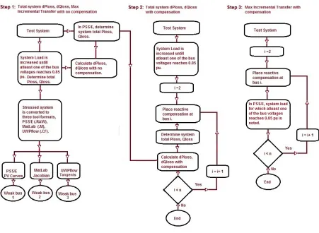
6 Steps 1, 2, 3 . . . 47

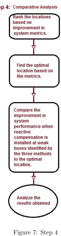
7 Step 4 . . . 48

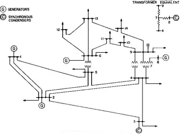
8 Modified IEEE 14 bus test system. . . 52

9 IEEE 30 bus test system. . . 54

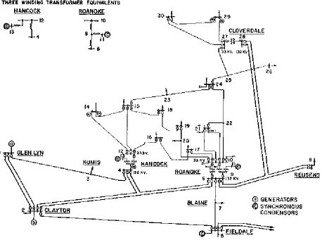
10 IEEE 57 bus test system. . . 58

11 The dQloss plot of 14 bus system. . . 66

12 The dPloss plot of 14 bus system. . . 67

13 The Maximum Incremental Transfer and size of reactive compensation at Maximum Incremental Transfer of 14 bus system. . . 67

14 The plot of improvement in Incremental Transfer per unit MVAR in 14 bus system. . . 68

23 Test system sparsities. . . 75

List of Tables

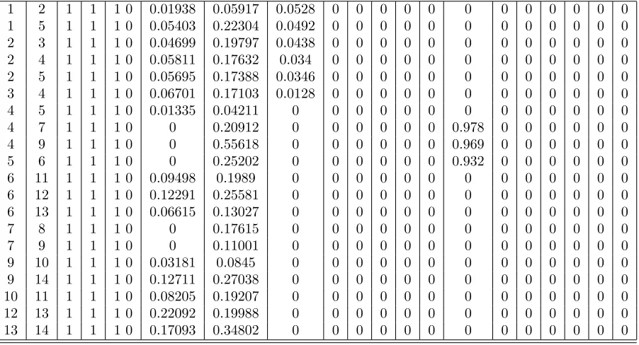
1 Bus data for14 bus test system . . . 53

2 Line data for 14 bus test system . . . 53

3 Bus data for IEEE 30 bus test system . . . 55

4 Line data for IEEE 30 bus test system . . . 56

5 Bus data for IEEE 57 bus test system . . . 59

6 Line data for IEEE 57 bus test system . . . 60

7 Continued..Line data for IEEE 57 bus test system . . . 61

8 Maximum Incremental Transfer (forVi ≥0.85pu),dPloss, anddQloss when no reactive compensation in the test systems . . . 64

9 14 bus system Voltages from PV Curves . . . 65

10 14 bus system Magnitude of Jacobian Elements from QV sensitivity Analysis 65 11 14 bus system greatest magnitude tangent vectors from Continuation Load Flow . . . 65

(8)

13 30 bus system Magnitude of Jacobian Elements from QV sensitivity Analysis 65 14 30 bus system greatest magnitude tangent vectors from Continuation Load

Flow . . . 65 15 57 bus system Voltages from PV Curves . . . 65 16 57 bus system Magnitude of Jacobian Elements from QV sensitivity Analysis 65 17 57 bus system greatest magnitude tangent vectors from Continuation Load

Flow . . . 65 18 Maximum Incremental Transfer (for Vi ≥ 0.85pu) for placement of Reactive

(9)

Abstract

Installation of reactive compensators is widely used for improving power system voltage

stability. Reactive compensation also improves the system loading margin resulting in more

stable and reliable operation. The improvements in system performance are highly

depen-dent on the location where the reactive compensation is placed in the system. This paper

compares three load flow analysis methods - PV curve analysis, QV sensitivity analysis, and

Continuation Load Flow - in identifying system weak buses for placing reactive

compensa-tion. The methods are applied to three IEEE test systems, including modified IEEE 14-bus

system, IEEE 30-bus system, and IEEE 57-bus system. Locations of reactive compensation

and corresponding improvements in loading margin and voltages in each test system obtained

by the three methods are compared. The author also analyzes the test systems to locate

the optimal placement of reactive compensation that yields the maximum loading margin.

The results when compared with brute force placement of reactive compensation show the

relationship between effectiveness of the three methods and topology of the test systems.

Keywords: Reactive Power, Static Voltage Stability, Placement, Load Flow Analysis,

(10)

1 Introduction

This chapter provides an overview of the evolution and establishment of

mod-ern power systems. Various aspects of power systems including load flow techniques, voltage

stability, voltage stability analysis techniques, and loading margin in particular are

intro-duced. A historical review of voltage stability analysis of power systems and methods of

volt-age stability analysis are presented. This thesis presents a comparative analysis of techniques

in load flow analysis for steady state voltage stability and loading margin improvements.

The remainder of this chapter includes an overview of modern power systems in

subsection 1.1, power system stability in subsection 1.2, voltage stability of power system in

subsection 1.3, voltage stability analysis methods in subsection 1.4, and practical techniques

for prevention of voltage collapse in subsection 1.5. The specific scope of this thesis is

represented in subsection 1.7 after providing a historical review of major blackouts caused

by voltage instability in subsection 1.6.

1.1 Modern Power Systems

The commercial use of electricity began in the late 1870s when arc lamps were

used for lighthouse illumination and street lighting [1]. The first complete electric power

system (comprising a generator, cable, fuse, meter, and loads) was built by Thomas Edison

-the historic Pearl Street Station in New York City which began operating in September 1882.

The load, which consisted entirely of incandescent lamps, was supplied at 110 V through an

underground cable system. Within few years similar systems were in operation in most large

(11)

motor loads were added to such systems.

Initially, dc systems were widely spread but by 1886 were completely

super-seded by ac systems. The reason being the increasingly apparent limitations of dc systems.

DC systems could deliver power only a short distance from the generators. To keep

trans-mission losses (I2_R_{) and voltage drops to acceptable levels, voltages had to be high for}

long-distance power transmission. Such high voltages were not acceptable for generation

and consumption of power, therefore a convenient means for voltage transformation became

a necessity. Some of the main reasons for the transition from dc to ac systems are easy

transformation of voltages thus providing the flexibility for use of different voltages for

gen-eration, transmission, and distribution, AC generators are much simpler than dc generators,

and AC motors are much simpler and cheaper than dc motors.

The decision to choose ac at Niagara Falls to transmit power about 30 km away

to Buffalo ended the ac versus dc controversy and established victory for the ac systems. In

early period of ac power transmission, frequency was not standardized. The use of many

different frequencies posed problems for interconnection. So eventually 60 Hz was adopted

as standard in North America, many other countries selected 50 Hz. The increasing need

for transmitting large amounts of power over longer distances created an incentive to use

progressively higher voltage levels. To avoid the proliferation of an unlimited number of

voltages, the industry has standardized voltage levels. The standards are 115, 138, 161, 230

KV for high voltage (HV) class, and 345, 500 and 765 KV for the extra-high voltage (EHV)

class [1].

Interconnection of neighboring utilities leads to improved security and

(12)

including the ones described above have been recognized from the beginning and

intercon-nections continue to grow leading to todays one big complex interconnected system with

almost all the utilities in United States and Canada. The design and secure operation of

such a system are indeed challenging problems.

In recent years, power demands around the world generally and particularly

in North America have experienced rapid increase due to the increase of customers’

require-ments. The report from Renewable Energy Transmission Company (RETCO) [2] about the

infrastructure situation of U.S. electric grids states that electricity consumption accounts for

40% of all energy consumed in the U.S. and the electricity demand grows significantly and

it will reach an increase rate of 26% by 2030.

Since 1982, growth in peak demand for electricity has exceeded transmission

growth by almost 25% every year. Yet spending on research and development is the lowest

of all industries [3]. Even with increase in demand, there has been chronic underinvestment

in getting energy where it needs to go through transmission and distribution which limits

grid efficiency and reliability. Since 2000, only 668 additional miles of interstate transmission

have been built [3]. As a result, system constraints worsen at a time when outages and power

quality issues are estimated to cost American business more than $100 billion on average

each year. Under these extreme conditions, the need for maintaining stable operation of the

grid is most important.

1.2 Power System Stability

Reference [4] defines power system stability as “the ability of an electric power

system, for a given initial operating condition, to regain a state of operating equilibrium

(13)

practically the entire system remains intact” . This definition applies to an interconnected

power system as a whole where the stability of a particular generator or a group of generators

is of interest. A remote generator may lose synchronism without causing cascading instability

of the whole system. Similarly, stability of particular loads or load areas may be of interest.

The power system is a highly nonlinear system that operates in a constantly

changing environment; loads, generator outputs and key operating parameters change

con-tinually. When subjected to a disturbance, the stability of the power system depends on

the initial conditions and nature of the disturbance. Power systems are subjected to a wide

range of disturbances, small and large. Small disturbances in the form of load changes occur

continually; the system must be able to adjust to the changing conditions and operate

satis-factorily. It must also be able to survive numerous disturbances of a severe nature, such as

a short circuit on a transmission line or loss of a large generator. A large disturbance may

lead to structural changes due to the isolation of the faulted elements.

However, it is impractical and uneconomical to design power system to be

stable for every possible disturbance [4]. The design contingencies are selected on the basis

that they have a reasonably high probability of occurrence. A stable equilibrium set thus has

a finite region of attraction; the larger the region, the more robust the system with respect to

large disturbances. The region of attraction changes continually with changes in operating

conditions of the power system.

Power system stability is a high dimensional and complex problem and in

order to deal with different types of instabilities occurring in the system it helps to make

simplifying assumptions to analyze specific types of problems using an appropriate degree of

(14)

stability problem is greatly facilitated by the classification of stability into various categories

[1]. The power system stability is mainly divided into rotor angle stability, frequency stability

and voltage stability. Voltage stability is explained in detail in subsequent sections as it is

the main focus of this thesis.

1.3 Voltage stability of Power System

Voltage stability is the ability of a power system to maintain steady

accept-able voltages at all buses in the system under normal operating conditions and after being

subjected to a disturbance [1]. A system enters voltage instability when a disturbance,

in-crease in load demand, or change in system condition causes a progressive and uncontrollable

drop in voltage. The main factor causing instability is the inability of the power system to

meet the demand for reactive power. A possible outcome of voltage instability is the loss

of load in an area, or tripping of transmission lines and other elements by their protective

systems leading to cascading outages. Voltage collapse is the process by which the sequence

of events accompanying voltage instability leads to a blackout or abnormally low voltages in

a significant part of the power system.

Voltage instability is mainly caused because of the loads; after a disturbance,

power consumed by the loads tends to be restored by the action of voltage regulators, tap

changing transformers, and thermostats. Restored loads increase the stress on high voltage

network by increasing the reactive power consumption and causing further voltage reduction.

A run-down situation causing voltage instability occurs when load dynamics attempt to

restore power consumption beyond the capability of transmission network and the connected

generation [1] [5].

(15)

experienced at least once [6]. This is caused by the capacitive behavior of the network as

well as by under excitation limiters preventing generators and/or synchronous compensators

from absorbing the excess reactive power. This instability is associated with instability of

the combined generation and transmission system to operate below some load level.

Voltage stability problems may also be experienced at HVDC links [7]. They

are usually associated with HVDC links connected to weak ac systems and may occur at

rectifier or inverter stations, and are associated with the unfavorable reactive power “load”

characteristics of the converters. The HVDC link control strategies have a significant

in-fluence on such problems, since the active and reactive power at the ac/dc junction are

determined by the controls. If the resulting loading on the ac transmission is relatively with

the time frame of interest being in order of one second or less.

It is useful to classify voltage stability into sub categories as discussed below:

1. Large - disturbance voltage stability is the ability of the system to maintain steady

per-missible voltages following large disturbances such as system faults, generator trips or

other circuit contingencies. This phenomenon is affected by the system and load

charac-teristics, and the interactions of both continuous and discrete controls and protections.

Determination of large signal voltage stability requires the examination of the nonlinear

response of the power system over a period of time sufficient to capture the performance

and interactions of devices such as motors, under load tap changers, generator field

cur-rent limiters, and speed governors. The study period of interest may extend from a few

seconds to tens of minutes. Therefore, long-term dynamic simulations are required for

analysis.

(16)

permissible voltages when subjected to small perturbations such as incremental changes

in system load. This form of stability is influenced by the characteristics of the load,

continuous controls, and discrete controls at a given instant of time. This concept is

useful in determining, at any instant, how the system responds to small system changes.

To identify the factors influencing stability, system equations can be linearized for the

analysis with appropriate assumptions.

The time frame of interest for voltage stability problems may vary from a few

seconds to tens of minutes. Therefore, voltage stability can be classified into short term and

long term on this basis.

1. Short - term voltage stability involves dynamics of fast acting load components such

as induction motors, electronically controlled loads, and HVDC converters. The study

period of interest is in order of several seconds, and the analysis requires solution of

appropriate system differential equations [4]. This analysis needs dynamic modeling of

loads.

2. Long - term voltage stability involves slower acting equipment such as tap-changing

transformers, thermostatically controlled loads, and generator and current limiters.

This analysis assumes that inter - machine synchronizing power oscillations have dumped

out, resulting in a uniform system frequency [8]. The focus is on slower and longer

du-ration phenomena that accompany large scale system upsets and on the resulting large,

sustained mismatches between the generation and consumption of active and reactive

powers. Long - term stability is usually concerned with system disturbances that involve

(17)

1.4 Methods of Voltage Stability Analysis

Voltage stability problems normally occur in heavily stressed systems. While

the disturbance leading to voltage collapse may be initiated by a variety of causes, the

underlying problem is a inherent weakness in the power system. The main factors other than

the design limitations of the system are generator reactive power/voltage control limits, load

characteristics, characteristics of reactive compensations devices, and the action of voltage

control devices such as under load tap changing transformers (ULTCs) [1].

The voltage stability analysis for a given system state involves the examination

of two concepts [9]:

1. Proximity to Voltage Instability: A measure of how close the system is to voltage

in-stability. Physical quantities such as load levels, active power flow through critical

interface and reactive power reserve can be used to measure the distance to instability.

The most appropriate measure for a given situation depends on the specific system and

the intended use of the margin. Considerations must be given to possible contingencies

such as line outages, loss of generating units or reactive power sources, etc.,

2. Mechanism of Voltage Instability: This includes the determination of the cause of

insta-bility including the key factors, voltage - weak areas and also finding out the measures

to improve stability.

The voltage instability problem is solved by many different methods, which

can be distinguished mainly in two groups: static and dynamic methods. Dynamic methods

apply real - time simulation in time domain using precise dynamic models for all instruments

(18)

eventually lead the system into voltage collapse. These methods mainly depend on the

solutions of large sets of differential equations created to describe the model characteristics of

electrical devices and their internal connections. Dynamic simulation is particularly effective

for detailed study of specific voltage collapse situations and coordination of protection and

time dependent action of controls. The dynamic simulation of large-scale power system is

time consuming and relies heavily on the computer’s performance.

The system dynamics influencing voltage instability are usually slow.

There-fore, static methods can be used to analyze many aspects of the problem. The static analysis

techniques allow examination of a wide range of system conditions and, if appropriately used,

can provide much insight into the nature of the problem and identify the key contributing

factors.

Static Analysis captures snapshots of system conditions at various time frames

along the time-domain trajectory. The electric utility industry has been widely dependent

on conventional power-flow techniques for static analysis of voltage stability. V-P and V-Q

curves are the most commonly used methods for voltage stability analysis. Although these

methods involve the establishment of stability characteristics by unrealistically stressing each

individual bus in the system. As a consequence, several techniques have been proposed for

voltage stability analysis using the static approach.

F. D. Galiana proposed a novel technique based on concept called the load

flow feasibility region (FR) and the steady state stability or feasibility margin (FM) [10].

The method does not rely on load flow solutions to give an estimate of how close the bus

injection vectors (P, Q, orV2) are to the boundary of FR thus avoiding the problems of

(19)

and the FM is a scalar ranging from 0 and 1. FM is a measure of the angle between the bus

injection vector and the closest injection vector on the the boundary of the FR along some

specified direction. A value of FM equal to 0 implies that the injections are on the boundary

of the FR and a value of FM greater than 0 indicates that the injections are inside the FR.

B. Gao, G. K. Morris, P. Kundur presented a technique to analyze the voltage

stability of large power systems using modal analysis technique [9]. The method computes

a specified number of the smallest eigenvalues and the associated eigen vectors of a reduced

Jacobian matrix and the associated bus, branch and generation participation factors. The

magnitude of the eigen values, each of which is associated with a mode of voltage/reactive

power variation determines the degree of stability of theith modal voltage. The smaller the

eigen value, closer the mode is to instability. The eigenvectors are used to describe the mode

shape and to information about the network elements and generators which participate

in each mode. The magnitude of eigen values provides a relative measure to instability.

However, they do not provide an absolute measure because of the nonlinearity of the problem

[1]. At any given operating condition, the system is stressed incrementally until it becomes

unstable to obtain a MW distance to instability. Modal analysis is then applied at each

operating point which gives the information about how stable the system is and how much

extra load the system can take. At the system’s voltage stability critical point, modal analysis

helps identify the voltage stability critical areas and elements participating in each mode.

The relation between voltage instability and multiple load flow solutions has

been investigated by Y. Tamura [11]. A set of N criteria are preset to differentiate between the

solution pair of the load flow to identify the stable and unstable one. The criterion used in this

(20)

for node injections and system parameters, and increase or decrease of stored energy of the

elements L and C in the electric power system due to small frequency disturbance raise.

Although the criterion 1 has some disadvantages in that it needs Jacobian J in the stable

system and involves uncertainty of sign{det J} when the even number of the eigenvalues

vary to the unstable mode, in the criteria 2 and 3 the property of solution can be judged at

any time point without the prior information.

The QV curve method [1], [27] has been used as a planning tool by many

utilities. QV curve may help engineers to identify critical buses in the system as well as the

reactive power injections needed at those buses to ensure voltage security. Pablo Guimaraes,

Ubaldo Fernandez, Tito Ocariz, Fritz W. Mohn, A. C. Zambroni de Souza presented a work

where they used QV and PV curves as planning tools of analysis [28]. In this work, a

planning tool based on some voltage stability criteria is proposed. They employed tangent

vectors to identify citical buses in the system and QV curves to identify the buses with least

and larger reactive power to obtain a good planning strategy. QV sensibility and curves have

been employed for voltage stability assessment [29], [30] in other power system studies.

V-Q sensitivity analysis has advantage that it provides voltage stability-related

information from a system-wide perspective and clearly identifies areas that have potential

problems. The elements of the Jacobian matrix gives the sensitivity between power flow and

bus voltage changes. The V-Q sensitivity at a bus represents the slope of the Q-V curve at

the given operating point. A positive V-Q sensitivity is indicative of stable operating, the

smaller the sensitivity, the more stable the system. As stability decreases, the magnitude of

the sensitivity increases, becoming infinity at the stability limit. A negative V-Q sensitivity is

(21)

operation [1]. A detailed mathematical description of Q-V sensitivity is given in further

chapters.

The PV curves represent the voltage variation with respect to the variation

of load active power. They are produced by a series of load flow solutions for different

load levels uniformly distributed, by keeping constant power factor. The active power is

proportionally incremented to the participating factors of each generator. PV curves are

widely used in industry for static voltage stability analysis of power system. The PV curves

are plotted for each bus and the bus which reaches the stability margin is identified as the

weak bus. A detailed mathematical description of the PV curves and how they are derived

is given in further chapters. S. Corsi and G. N. Taranto presented a paper elaborating the

understanding of dependence of the shape of the “nose” of a Power-Voltage (PV) curve in a

EHV bus, by the power system dynamics [13]. The paper showed in detail the involvement

of control loops in voltage instability phenomenon and their effect on the shape of PV curve.

Venkataraman Ajjarapu, Colin Christy presented a method of finding a

con-tinuum of power flow solutions starting at some base load and leading to the steady state

stability limit (critical point) of the system [12]. The method uses reformulated power flow

equations with a load parameter as an additional parameter. The continuation algorithm is

then applied to the system of reformulated power flow equations. The process involves

pre-dictor and corrector steps to find the consecutive solutions, it remains well conditioned near

and beyond the stability limit consequently avoiding the problems of conventional power-flow

which are prone to convergence problems at operating condition near the stability limit. A

detailed mathematical description of the method is given in further chapters.

(22)

analysis [24] where the system tangent vectors were computed using inverse of the Jacobian

matrix. In this work, normalized tangent vectors were compared to the eigenvectors to whom

the same normalization was applied. A. C. M. Valle later presented a paper where he used

tangent vectors and eignevectors in power system voltage collapse analysis [25]. In this work,

a relation between the tangent vectors and eigenvectors is used to converge to the bifurcation

point sooner and to identify the most sensible bus and the generator which most influence

the bus voltage oscillation.

B. Isaias Lima Lopes, A. C. Zambroni de Souza, and P. Paulo C. Mendes

presented a paper that talked about the use of tangent vectors as a tool for voltage collapse

analysis considering a dynamic model [26]. In this work, they employed the continuation

method for the power flow model to calculate the indices for each operating point and

the process is repeated for dynamic system model. The results are compared and showed

that dynamic model may be more pessimistic for loading margin evaluation, since the static

model tends to produce results more conservative. They conclude that monitoring the indices

during the system load increase may not be enough to identify the voltage collapse point.

However, tangent vector presents a better behavior than the least eigenvalue, since latter is

associated with a sudden variation at the voltage collapse point.

Continuation load flow has been used in several instances for steady state power

system analyses and to obtain system tangent vectors [28] [31] [32] [33]. A. Sode-Yome, N.

Mithulananthan, K. Y. Lee presented a paper comparing various FACTS devices [14]. They

used several performance measures including PV curves, voltage profiles, and power losses

are compared to evaluate their performance. Continuation load flow was used for steady

(23)

paper investigates both placement and sizing techniques for better choice of FACTS devices

for enhancing loading margin and static voltage stability.

1.5 Practical Techniques for Prevention of Voltage Collapse

Several measure could be taken to avoid voltage collapse, system design

mea-sures and system operating meamea-sures are the common practices for this purpose [1]. System

design measures that can be taken to avoid voltage collapse are:

1. Application of Reactive Power-Compensating devices: Adequate stability

mar-gins should be maintained by selecting the appropriate sizes, ratings, and locations

for reactive compensation devices based on detailed studies covering the most onerous

system conditions for which the system is required to operate satisfactorily

2. Control of Network Voltage and Generator Reactive output: Generator AVR

regulates voltages on the high-tension side of the step-up transformer moving the point

of constant voltage electrically closer to the loads. A secondary outer control loop with

response time of about 10 seconds is used to regulate network side voltage.

3. Coordination of Protections/Controls: Lack of coordination between equipment

protections/controls and power system requirements could lead to voltage collapse,

ad-equate coordination should be ensured based on dynamic simulation studies. Adad-equate

control measures should be provided for relieving any overload conditions before

iso-lating equipment from the system, tripping of equipment should be the last resort to

prevent an overloaded condition.

4. Control of Transformer Tap Changers: Tap changing transformers are used to

(24)

and distribution system characteristics must be employed to improve ULTC control

[1]. Microprocessor-based ULTCs on the other hand provide unlimited flexibility in

implementing control strategies so as to take advantage of the load characteristics.

5. Undervoltage Load Shedding: Load shedding based on carefully designed schemes

to cater unplanned or extreme situations is a low cost means of preventing widespread

system collapse. It is employed in both underfrequency and undervoltage control, the

characteristics and locations of loads to be shed are more important for voltage problems

than they are for frequency problems [1].

System-operating measure that can be taken to avoid voltage collapse are:

1. Stability Margin: Maintaining adequate voltage stability margin by scheduling of

reactive power and voltage profiles could help avoid voltage collapse. All systems are

different and should be the parameters and degree of margin designed based on the

particular system.

2. Spinning Reserve: Maintaining adequate spinning reserves and switching in

capaci-tors by appropriately identifying the need to maintain the desired voltage profile.

3. Operators’ Action: Operators must be able to identify voltage stability-related

symp-toms and take remedial actions based on well designed strategies to prevent voltage

col-lapse. On-line monitoring and analysis could direct to appropriate preventive actions

so as to avoid voltage collapse situation.

1.6 Major Blackouts caused by Voltage Instability

Power industries were initially dedicated as service oriented and driven

(25)

deregulation was introduced to improve the managerial efficiency. This lead to a

compet-itive market structure with increase in system utilization and it also increased the risk on

system operations by stressing the power systems and reducing the predictability of

opera-tions. Interconnection with neighboring countries or sub systems made the network stronger,

however this also increases the area covered by the network thus increasing risk on external

interferences. This also increases the risk of having many disturbances at the same time

therefore makes it difficult to design the system to sustain N-1 contingency and reduce the

security of the power system.

The first officially reported major blackout was the Northeast power failure

on 9th November 1965. The backup protection tripped one of the five line connecting the

northeast and southwest under heavily loaded conditions [15]. This eventually led to the

tripping of rest of the four lines diverting 1700 MW of power which eventually led to total

system collapse. It was also identified that there was not enough spinning reserve kept at

the time the blackout was initiated. The blackout affected 30 million people and New York

City was in darkness for 13 hours. The 13th July 1977 collapse of Con Edison System left

8 million people in darkness, including New York City for periods from 5 to 25 hours [15].

Lack of preparation for major emergencies, operating errors, questionable system design,

and equipment malfunction with a combination of natural events were recognized as the

causes of the event. Imperfect operation of protective equipment resulted in three of four

lines tripping which resulted in transmission ties overloading eventually opening them which

led to total system operation failure.

On 23rd_{July 1987, a power failure occurred in Tokyo, Japan due to insufficient}

(26)

GW, the 1.52 GW reserve was insufficient for the unusual high peak demand due to extreme

hot weather [15]. Widely used constant power characteristic loads such as air conditioners

reduced the network voltage rapidly and caused dynamic voltage instability. The Western

North American power system reported an interruption leading to failure on 2nd _{July 1996.}

It was initiated with a flashover to a tree which created a short circuit on a transmission line

causing a 2 GW power interruption. This line was a series compensated with a capacitor, the

loss of power transfer caused voltage depression and thus tripped a few hydro generators due

to high field current causing a voltage decay. To prevent further down process, five islanded

sub systems were formed with controlled and uncontrolled load shedding.

50 million people were affected on 14th August 2003 in US and Canadian due

to a blackout which interrupted 63 GW load. In this event 400 transmission lines and 531

generating units at 261 power plants tripped. The major reason was found to be insufficient

reactive power, which lead to voltage instability. Failure was initiated with tripping voltage

regulator due to over excitation and when the operators tried to restore the regulators,

generators which were generating high reactive power were tripped. Finally, tripping of a tie

line lead to cascading blackout of the entire region. Several other blackouts were reported

over the past decade including 23rd_{September 2003 blackout in Europe, the Swedish/Danish}

system, 28th_{September 2003 blackout in Italy, and a major interruption in Victoria, Australia}

on 16th _{January 2007 that interrupted service to 480,000 customers.}

Operator action and load shedding could have greatly reduced the impact in

most of the situations listed above [15]. Gathering and analysis of technical information on

the root cause of blackouts, development of load shedding schemes with technical

(27)

on requirement of the system operator’s training are few of the measures that could avoid a

(28)

1.7 Scope and Contribution of Thesis

Over the years, various methods have been used to identify the weak buses of a

system for reactive power installation in several studies. This thesis is an investigation into

whether there are any differences in improvement of the system design and consequently

performance caused by the use of different load flow analysis techniques to identify the

location for installing reactive compensation. The investigation conducted in this thesis

consists of comparing three methods namely Continuation Load Flow, PV Curve Analysis,

and QV sensitivity analysis to identify the weak buses in multiple systems and a reactive

compensation is installed at these locations. Various metrics including maximum loading

margin and the system differential active and reactive power losses are compared to the

results of installing a reactive compensation at the optimal location obtained from

brute-force to identify the method(s) that identifies a location that gives better results compared

to other method(s).

Load flow equations are multi dimensional and coupled set of equations, which

usually are solved using iterative techniques. Several techniques have been developed for this

purpose and the results obtained are analyzed using even more techniques. PV curve analysis

and QV sensitivity analysis are obtained from the traditional load flow. Continuation load

flow is more recent developed method of load flow analysis which gives other sensitivity

information useful in system analysis.

PV curves are the plots of real power and voltage at some critical buses which

help determine the static voltage stability of the system. For any given loading condition the

bus voltage has two possible values except at the stability limit where the load flow equations

(29)

is of utmost importance to never operate the system at unstable voltage levels, this could

cause a serious black out though uncontrollable collapse of voltage levels in the system. PV

curves help identify the operating voltages for different levels of real power requirement and

also specify the weak buses in the system which are prone to voltage instability.

QV sensitivity analysis is the change in bus voltage with injection or absorption

of reactive power (Q) at any bus. For a system to be in stable operating mode, it is necessary

that all the buses in the system have a positive QV sensitivity. The degree of sensitivity can

be observed in the elements of the Jacobian matrix of load flow equations. For a given set

of parameters (P, Q, V and θ), the magnitude of elements of the Jacobian matrix identify the

buses that are highly sensitive to Q. The small the QV sensitivity, the more stable the bus

is. As the stability decreases, the magnitude of QV sensitivity increases becoming infinite

at stability limit. However, even a small negative QV sensitivity is an indicative of highly

unstable operation.

Continuation load can be used to compute the load flow solutions beyond

the stability limit of the system which conventional load flow techniques fail to provide.

This is due to the convergence problems of the Jacobian matrix in conventional load flow

methods, which the Continuation load flow method over comes by employing a prediction

and correction of tangent vectors at a given solution of the load flow equations. The method

provides very useful sensitivity information at no additional cost at all. The magnitudes of

the tangent vectors at a given solution provide the sensitivity information of all the buses.

The greater the magnitude, the more unstable the bus is in the system.

Reactive power installation is a widely used technique for voltage stability and

(30)

plays a crucial role in determining the improvement that can be obtained in the system.

Installation of reactive compensation at weak buses of the system has shown to improve

the system voltage stability and loading margin [14]. However, the definition of a weak bus

changes with the load flow and sensitivity analysis used. Thus, it is important to identify the

differences in improvement of system performance based on the analysis method employed.

The measure of improvement in system performance is an important aspect

for analysis purposes. Several metrics could be used to achieve this purpose. Differential

real and reactive power losses of the system and maximum loading margin of the system are

the metrics used in this thesis to measure the system performance.

The active and reactive power losses are related to the bus voltage angle and

magnitude stability of the system. It can be observed from the system Jacobian matrix that

the voltage angle is dependent on the real power available at a bus and the voltage magnitude

is dependent on the reactive power available at a bus. Reducing the losses increases the

available real and reactive power at a bus, thus improving the voltage stability.

Maximum loading margin of a system is the load beyond which increase in load

will drive the system to instability. The system is operated by maintaining sufficient margin

from this maximum loading margin so as to always keep the system in stable operating

conditions. An increase in the system maximum loading margin will provide an improvement

in the load which the system can supply and still keep a sufficient margin from the maximum

loading margin.

In further chapters, various load flow methods, analysis techniques, and metrics

that will be used in this thesis will be discussed in detail. Then methodology is proposed

(31)

installation. The methodology is then applied to various test systems and the results are

(32)

2 Mathematical Modeling

Mathematical modeling of the load flow problem, various load flow analysis

techniques along with stability analysis techniques are discussed in this chapter.

2.1 Load Flow Problem

The main objective of solving the load flow problem is calculation of the power

flows and voltages of a transmission network for specified bus conditions. These calculations

are required for both steady state and dynamic analysis as well. The bus classification are

as described below:

1. Variables: Voltage magnitude, Voltage phase angle, real power requirement, and

re-active power requirement.

2. Voltage-Controlled (PV) bus: Voltage magnitude and active power are known

quan-tities for this kind of buses, reactive power limits are specified as well.

3. Load (PQ) bus: Active and reactive power requirements are the known quantities at

this type of bus locations.

4. Slack (Swing) bus: Voltage magnitude and phase angle are the known quantities for

this type of bus, there must be at least one bus with unspecified P and Q because of

the unknown P and Q losses in the system.

The network equations in terms of the node admittance matrix are written as

(33)

               ˜ I1 ˜ I2 ˜ I3 .. . ˜ In                =               

Y11 Y12 Y13 . . . Y1n

Y12 Y22 Y23 . . . Y2n

Y31 Y32 Y33 . . . Y3n

..

. ... ... . .. ...

Yn1 Yn2 Yn3 . . . Ynn

                              ˜ V1 ˜ V2 ˜ V3 .. . ˜ Vn                (1) Where

n is the total number of nodes

Yii is the self admittance of node i

Yij is the mutual admittance between nodes i and j

˜

Vi is the phasor voltage to ground at nodei

˜

Ii is the phasor current flowing into the network at node i

The set of equations 1 would be linear if ˜I were known, however the current

injections are not known for most nodes. The relations between the node currents, P, Q,

and V are as follows:

˜

Ii =

Pi−jQi

˜

V_i∗ (2)

Due to non linearity of the problem, load flow equations are solved iteratively.

Several techniques have been developed to solve the set of equations, [16] presents various

methods developed over the years.

2.2 Load Flow Analysis Techniques

(34)

This is an iterative approach proposed by Seidel in 1874 (Academy of Science,

Munich). The equation 2 is rewritten as follows:

Pi−jQi

˜

V_i∗ =Yii

˜

Vi + n

X

k=1,k6=i

YikV˜k (3)

The voltage ˜Vi may be expressed as

˜

Vi =

Pi−jQi YiiV˜i∗

− 1

Yii n

X

k=1,k6=i

YikV˜k (4)

For a load (PQ) bus, P and Q are know, and equation 4 is used to compute the

voltage ˜Vi by using updated voltages as soon as they are available i.e., for the Pth iteration,

the bus voltages used for computing voltageViat busiareV1p, V

p

2, . . . , V

p i−1, V

p−1

i , V p−1

i+1 , . . . , Vp

−1

n .

If ith _{bus is a generator bus, the reactive power to be generated is calculated}

using equation 5. If the computed Qi is within the Q limits of the generator, the value is

used in equation 4 to compute the updated value of Vi. The value of the voltage is forced

to be the specified value by multiplying the real and imaginary parts of the equation 4 with

ratio of specified value of the magnitude of generator voltage to the magnitude of its updated

value.

Qi =−Im[ ˜Vi∗ n

X

k=1

YikV˜k] (5)

On the other hand, if the computed Qi exceeds the Q limits of the generator,

it is set to the maximum or minimum limit based on whether it is above or below the limits

(35)

The iterations are continued until the real and imaginary components of

volt-ages at each bus computed by successive iterations converge to a pre specified tolerance. The

Gauss-Seidel method has slow convergence because of weak diagonal dominance of the node

admittance matrix. Acceleration factors are often used to speed up the convergence:

˜

Vnew

k =Vk˜old+c( ˜Vknew−Vk˜old) (6)

Where c is the acceleration factor, typically on the order of 1.4 to 1.7.

2.2.2 Newton-Raphson (N-R) Method:

Newton-Raphson method is an iterative technique used for solving a set of

non-linear equations. Let equation 7 represent a set of equations with n unknowns:

f1(x1, x2, . . . , xn) =b1

f2(x1, x2, . . . , xn) =b2

f3(x1, x2, . . . , xn) =b3

. . . .

fn(x1, x2, . . . , xn) =bn

(7)

The process stats with an initial guess of all the n unknowns x0

1, x02, x03, . . . , x0n

and if ∆x1,∆x2,∆x3, . . . ,∆xn are the corrections necessary to the initial guess so that the

(36)

f1(x01+ ∆x1, x02 + ∆x2, . . . , x0n+ ∆xn) = b1

f2(x01+ ∆x1, x02 + ∆x2, . . . , x0n+ ∆xn) = b2

f3(x01+ ∆x1, x02 + ∆x2, . . . , x0n+ ∆xn) = b3

. . . .

fn(x01+ ∆x1, x02 + ∆x2, . . . , x0n+ ∆xn) = bn

(8)

Each of the above equations can be expanded using Taylor’s theorem. The

expanded form of the ith _{equation is}

fi(x01 + ∆x1, x02+ ∆x2, . . . , x0n+ ∆xn) =fi(x01, x 0 2, x

0 3, . . . , x

0

n,)

+δfi

δx1

0

∆x1 +

δf_i

δx2

0

∆x2 +

δf_i

δx3

0

∆x3+. . .+

δf_i

δxn

0

∆xn

+ terms with higher powers of ∆x1,∆x2,∆x3, . . . ,∆xn (9)

The higher order terms in equation 9 can be ignored if the initial guess is close

to the true solution. The resulting linear set of equations in matrix form is

              

b1−f1(x01, x02, x03, . . . , x0n,)

b2−f2(x01, x02, x03, . . . , x0n,)

b3−f3(x01, x02, x03, . . . , x0n,)

. . . .

bn−fn(x01, x02, x03, . . . , x0n,)

               =                 δf₁ δx1 0 δf₁ δx2 0 δf₁ δx3

0 . . .

δf₁ δxn 0 δf₂ δx1 0 δf₂ δx2 0 δf₂ δx3 0

. . . δf2 δxn 0 δf₃ δx1 0 δf₃ δx2 0 δf₃ δx3 0

. . . δf3 δxn 0 . . . .. . . . δf_n δx1 0 δf_n δx2 0 δf_n δx3 0

. . . δfn δxn 0                               

∆x1

∆x2

∆x3

.. .

∆xn

(37)

Or

∆f =J∆x (11)

Where J is referred to as the J acobian. If the estimatedx0₁, x0₂, x0₃, . . . , x0_nwere

exact, then ∆f and ∆x would be zero. However, asx0

1, x02, x03, . . . , x0n are only estimates, the

errors ∆f are finite. Equation 10 represents a linear relationship between the errors ∆f and

the corrections ∆x through the Jacobian of the simultaneous equations. A solution for ∆x

can be obtained by applying any suitable method for the solution of a set of linear equations.

Updated values of x are calculated from equation 12

x1_i =x0_i + ∆xi (12)

The iterations have quadratic convergence and they are carried out until the

errors ∆fi are lower than a specified tolerance. The Jacobian has to be recalculated at each

step.

2.2.3 Application of the N-R method to power-flow solution:

In order to apply the Newton-Raphson method to power-flow equations, the

complex equations represented by equation 3 are rewritten as two real equations in terms of

two real variables. For any node i, we have

˜

Si =Pi+jQi = ˜ViI˜i∗ (13)

From equation 1,

˜

Ii = n

X

m=1

˜

(38)

Substituting ˜Ii given by equation 14 in equation 13 yields

Pi+jQi = ˜Vi n

X

m=1

(Gim−jBim) ˜Vm∗ (15)

The product of phasors ˜Vi and ˜Vm∗ may be expressed as

˜

ViV˜m∗ = (Viejθi)(Vmejθm) =ViVmej(θi−θm)=ViVm(cosθim+jsinθim)

where(θim=θi−θm)

(16)

The expressions for Pi and Qi may be written as follows:

Pi =Vi n

X

m=1

(GimVmcosθim+BimVmsinθim)

Qi =Vi n

X

m=1

(GimVmsinθim−BimVmcosθim)

(17)

Thus P and Q at each node is represented as a function of voltage magnitude

V and angle θ of all nodes.

If the active and reactive powers at each bus are specified, using subscript sp

(39)

P1(θ1, θ2, . . . , θn, V1, V2, . . . , Vn) = P1sp

P2(θ1, θ2, . . . , θn, V1, V2, . . . , Vn) = P2sp

. . . .

Pn(θ1, θ2, . . . , θn, V1, V2, . . . , Vn) = Pnsp

Q1(θ1, θ2, . . . , θn, V1, V2, . . . , Vn) =Qsp1

Q2(θ1, θ2, . . . , θn, V1, V2, . . . , Vn) =Qsp2

. . . .

Qn(θ1, θ2, . . . , θn, V1, V2, . . . , Vn) = Qspn

(18)

Following the general procedure described earlier for the application of the N-R

method (Equation 10), we have

                  

P₁sp−P1(θ10, . . . , θn0, V10, . . . , Vn0)

. . . .

P_nsp−Pn(θ01, . . . , θn0, V10, . . . , Vn0)

Qsp₁ −Q1(θ01, . . . , θ0n, V10, . . . , Vn0)

. . . .

Qsp

n −Qn(θ10, . . . , θn0, V10, . . . , Vn0)

                   =                     δP1 δθ1

. . . δP1 δθn

δP1

δV1

. . . δP1 δVn

. . . .

δPn δθ1

. . . δPn δθn

δPn δV1

. . . δPn δVn δQ1

δθ1

. . . δQ1 δθn

δQ1

δV1

. . . δQ1 δVn

. . . .

δQn δθ1

. . . δQn δθn

δQn δV1

. . . δQn δVn                                       

∆θ1

.. .

∆θn

∆V1

.. .

∆Vn

                   (19)     ∆P ∆Q     =     δP δθ δP δV δQ δθ δQ δV     J acobian     ∆θ ∆V     (20)

(40)

terms corresponding to ∆Q and ∆V would be absent for each of the PV buses. Thus the

Jacobian would have only one row and one column for each PV bus.

2.2.4 PV Curve Analysis:

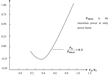
The V-P and Q-V characteristics have been widely used for the voltage stability

analysis. Figure 1 shows the relation between receiving end voltage and power for load at

different power factors.

Figure 1: TheVR−PR characteristics of a power system for different load power factors.

VP characteristic curves are produced by using a series of power flow solutions

for different load levels. The analysis involves the increase of P i.e. real power demand in

a particular area and voltage magnitude (V) is observed at some critical load buses and

then curves for those particular buses will be plotted to determine the voltage stability of a

(41)

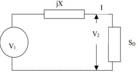
To explain P-V curve analysis let us assume two-bus system with a single

generator, single transmission line and a load, as shown in figure 2.

Figure 2: Two bus represetation model.

The complex load assumes the form as shown in equation 21 where V1 is the

sending end voltage and V2 is the receiving end voltage and cosθ is the load power factor.

S12=P12+jQ12 (21)

From the Figure 2, the following equations can be derived:

P12=|V1|2G− |V1||V2|Gcos(θ1−θ2) +|V1||V2|Bsin(θ1−θ2)

Q12=|V1|2B − |V1||V2|Bcos(θ1−θ2)− |V1||V2|Gsin(θ1−θ2)

(22)

Let G=0, then

P12=|V1||V2|Bsin(θ1−θ2)

Q12=|V1|2B− |V1||V2|Bcos(θ1−θ2)

(23)

(42)

SD =PD +jQD =−(P21+jQ21)

PD =−P21 =−|V1||V2|Bsin(θ2−θ1) = |V1||V2|Bsin(θ1−θ2)

QD =−Q21=−|V2|2B− |V1||V2|Bcos(θ2 −θ1) =−|V2|2B− |V1||V2|Bcos(θ1−θ2)

(24)

Defining θ12=θ1−θ2

PD =|V1||V2|Bsinθ12

QD =−|V2|2B +|V1||V2|Bcosθ12

(25)

From the figure, we can also express:

SD =|V2||I|ejφ =|V2||I|(cosφ+jsinφ)

=PD(1 +jtanφ) = PD(1 +jβ), whereβ=tanφ

QD =PDβ =−|V2|2B+|V1||V2|Bcosθ12

(26)

Equating the expressions for PD and QD, we have

(|V2|2)2+

h2P_Dβ

B − |V2|

2₊ PD

B2[1 +β

2_]i_{= 0} ₍₂₇₎

Equation 27 is a quadratic in|V2|2, eliminatingθ12and solving the second order

(43)

|V2|2 =

1−βPD ±

p

[1−PD(PD + 2β)]

2 (28)

As seen in equation 28, the voltage at the load bus is affected by power delivered

to the load, the reactance of the line, and power factor of the load. It can be seen that the

equation 28 has two solutions for a given set of parameters. One of them corresponds to

stable operation and the other corresponds to unstable operation of the system.

In figure 1, the nose of the curve corresponds to the maximum loading point

of the system. For a given loading pattern, the PV curves are plotted for selected PQ buses.

This reveals the maximum loading margin of the system after which at least one of the

bus voltages becomes unstable, which means the system is no longer in stable operating

condition. The bus which enters voltage instability first for a given loading pattern can be

identified as the weak bus of the system. Installation of reactive compensation devices at

such locations can greatly improve the voltage stability and loading margin of the system.

2.2.5 QV Curve Analysis:

Voltage stability is affected considerably by the variations in Q (reactive power

consumption) at loads. A more useful characteristic for voltage stability analysis is the

Q-V relationship, which shows the sensitivity of bus voltage with respect to reactive power

injections and absorptions. A system is voltage stable if V-Q sensitivity is positive for all

the buses and is unstable if it is negative for at least one bus.

Figure 3 shows a typical VR−QR characteristic curve of power system.

The base case operating point of the system is represented by the X-intercept

(44)

Figure 3: The VR−QR characteristics of a power system.

When a solution is reached using N-R method, we have a linearized model

around the given operating point.

J     ∆θ ∆V     =     ∆P ∆Q    

Where [J] =     δP δθ δP δV δQ δθ δQ δV     (29)

The elements of the Jacobian matrix represent the system sensitivity

informa-tion, i.e., expected small change in bus voltage angle (θ) and voltage magnitude (V) for small

changes in P and Q. System voltage stability is affected by both P and Q. In this analysis,

(45)

the incremental relationship between Q and V. Based on these considerations, in equation

29, let ∆P = 0 , we have

∆Q=JR∆V

where JR = [JQV −JQθJP θ−1JP V]

(30)

Where JR is the reduced Jacobian matrix. From equation 30, we may write

∆V =J_R−1∆Q (31)

The matrix J_R−1 is the reduced V-Q Jacobian. Its ith _{diagonal element is the}

V-Q sensitivity at bus i. For computational efficiency, the V-Q sensitivities are computed

from equation 30.

The V-Q sensitivity of a bus represents the slope of the Q-V curve at the

given operating point. A positive V-Q sensitivity is an indicative of stable operation; the

smaller the sensitivity, the more stable the system. As stability decreases, the magnitude

of the sensitivity increases, becoming infinite at stability limit. A negative V-Q sensitivity

however, is an indicative of unstable operation, even a small negative sensitivity represents

very unstable operation.

2.2.6 Continuation Load Flow Analysis:

The Jacobian matrix of power flow equations becomes singular at the voltage

stability limit. Consequently, conventional power-flow algorithms are prone to convergence

(46)

this problem. It does so by reformulating the power-flow equations so that they remain

well-conditioned at all loading conditions.

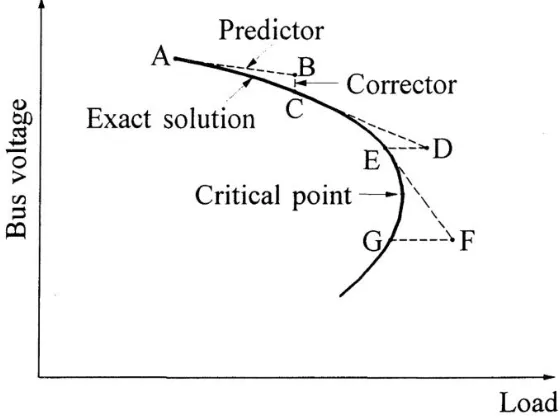
The continuation power-flow analysis uses an iterative process involving

pre-dictor and corrector steps as depicted in figure 4.

Figure 4: Representation of a typical continuation power-flow process.

From a know initial solution (A), a tangent predictor is used to estimate the

solution (B) for a specified patter of load increase. The corrector step then determines

the exact solution (C) using a conventional power-flow analysis with system load assumed

to be fixed. Successive solutions are obtained by the same predictor and corrector steps.

Eventually, the system reaches a loading condition where a corrector step with loads fixed

would not converge; therefore, a corrector step with fixed voltage at the monitored bus is

applied to find the exact solution (E).

(47)

The injected powers for ith _{bus of an} _n_{-bus system as represented by equation}

17

Pi =Vi n

X

m=1

(GimVmcosθim+BimVmsinθim)

Qi =Vi n

X

m=1

(GimVmsinθim−BimVmcosθim)

(17)

The equations for the real and reactive power injections at bus i are given by

equation 32

Pi =PGi−PDi

Qi =QGi−QDi

(32)

The subscript G and D denote generation and demand respectively for bus i.

A load parameter λ is introduced as an additional parameter in equations 32

to simulate load change in the system.

Pi =PGi−(PDi+λ(P∆base))

Qi =QGi−(QDi+λ(Q∆base))

(33)

In equation 33, P∆base and Q∆base are given quantities of powers chosen to scale λ

appro-priately. The reformulated power-flow equations, with provision for increasing generation as

(48)

F(θ, V) = λK (34)

Where

λ is the load parameter

θ is the vector of bus voltage angles

V is the vector of bus voltage magnitudes

K is the vector representing percentage load change at each bus

The equation 34 may be rearranged as equation 35 and is solved by specifying

a value forλ as shown in equation 36. Whereλ = 0 represents the base load condition, and

λ=λcritical represents the critical load of the system.

F(θ, V, λ) = 0 (35)

0≤λ≤λcritical (36)

Predictor Step:

To find the solution of the set of equations represented by equation 35, a linear

approximation is used by taking an appropriately sized step in direction tangent to the

(49)

Fθdθ+FVdV +Fλdλ = 0

or

Fθ FV Fλ

       dθ dV dλ        = 0 (37)

The set of equations 37 have one additional unknown i.e.,λthe load parameter.

Hence, one more equation is needed to solve these equations. This is satisfied by setting one

of the components of the tangent vectors to +1 or -1. This component is referred to as

continuation parameter. Setting one of the tangent vector components +1 or -1 imposes

a non-zero value on the tangent vector and makes the Jacobian matrix nonsingular at the

critical point. With the additional equation, we have



  

Fθ FV Fλ

ek            dθ dV dλ        =     0 ±1     (38)

Where ek is the appropriate row vector with all elements equal to zero except

the kth _{element (corresponding to the continuation parameter) begin equal to 1. Initially,}

the load parameterλ is chosen as the continuation parameter. Subsequently, the parameter

with greatest rate of change at a given solution is chosen as the continuation parameter.

This is due to the fact that the use of λ as the continuation parameter near critical loading

conditions can cause the solution to diverge if the estimate exceeds the maximum load.

(50)

may diverge if large steps in voltage change are used. A good practice is to choose the

continuation parameter as the state variable that has the greatest rate of change near the

given solution. If the parameter is increasing +1 is used, if it is decreasing -1 is used in the

tangent vector equation 38.

The tangent vectors can be obtained by solving equation 38. Once these are

solved for, the prediction can be made as follows

       θ V λ        p+1 =        θ V λ        p +σ        dθ dV dλ        (39)

Where the superscript p+ 1 denotes the next predicted solution. The step

size σ is chosen so that the predicted solution is within the radius of the convergence of the

corrector. If for a step size the solution could not be found, a smaller step size is chosen.

Corrector Step:

The original set of equations 35 is augmented by one equation that specifies

the state variable selected as the continuation parameter. This gives



  

F(θ, V, λ)

xk−η



  

= [0] (40)

Where xk is the state variable chosen as continuation parameter and η is the

predicted value of this state variable. Equation 40 can be solved using a slightly modified

(51)

The continuation power-flow analysis can be continued beyond the critical

point and thus obtain solutions corresponding to the lower portion of the V-P curve. It

should be noted that the tangent component of λ is positive before the critical point is

reached, zero at the critical point, and negative beyond this point. Therefore the sign of dλ

shows whether the critical point is reached or not.

Sensitivity Information:

In continuation process, the tangent vector proves useful in describing the

direction of the solution path. If one looks at the elements of the tangent vector as differential

changes in the state variables (dVi and dδi) in response to a differential change in system

load (Cdλ, where C is some constant), the potential for a meaningful sensitivity analysis

becomes apparent [12].

It can be observed that the voltage at bus i is affected by load changes at

not only itself but at other buses as well. Hence the best method for deciding which bus is

nearest to its voltage stability limit is to find the bus with the largest dVi

dPT otal

, wheredPT otal

is the differential change in active load for the whole system.

Using the reformulated power flow equations, the differential change in active

system load is as follows:

dPT otal =

X

n

dPLi =

X

n

[kLiS∆Basecosψi]dλ

= [S∆Base

X

n

kLicosψi]dλ=Cdλ

(52)

Thus, the weakes bus would be busj : dVj dPT otal

= dVj Cdλ =max h dV1 Cdλ , dV2 Cdλ , . . . , dVn Cdλ i (42)

Since the value of Cdλ is same for eachdV element in a given tangent vector,

the weakest bus can be identified as the bus with largest dV component.

2.3 Summary

Both the load flow techniques Newton-Raphson method and Continuation load

flow method have been discussed in detail. The analysis methods PV curve analysis, QV

sensitivity analysis, and Continuation load flow analysis have also been explained in this

chapter. In the next chapter, a method of analyzing the improvement in system performance

is introduced and it is then applied to various test systems in further chapters. Results are

Comparative Analysis of Load Flow Techniques for Steady State Loading Margin and Voltage Stability Improvement of Power Systems

ScholarWorks@UNO

ScholarWorks@UNO

Comparative Analysis of Load Flow Techniques for Steady State

Comparative Analysis of Load Flow Techniques for Steady State

Loading Margin and Voltage Stability Improvement of Power

Loading Margin and Voltage Stability Improvement of Power

Systems

Systems

Acknowledgements

Contents

List of Figures

List of Tables

Abstract

1

Introduction

2

Mathematical Modeling