Design of Flux Observer for Induction Machine
Using Adaptive Control Theory
Sharad Salunke
Department of Electrical & Electronics Engineering, Sagar Institute of Research & Technology, Bhopal (M.P.), India Email: [email protected]
Ashish Sharma
Department of Electronics and Instrumentation, SGSITS, Indore (M.P.), India
Email: [email protected]
Abstract
—
In the sensorless speed control of induction motors with direct field orientation, the rotor flux and speed information are dependent on the observers. However, the exact values of the parameters that construct the observers are difficult to measure and changeable with respect to the operating conditions. When the motor parameters are changed and thus different from the preset values, the estimated flux will deviate from the real values. To make flux estimation robust to parameter variations, a flux observer is proposed in the paper. The stability of the method is proven by Lyapunov theory.I. INTRODUCTION
Larger industrial applications require high performance motion control with four quadrant operation including field weakening, minimum torque ripple, rapid speed recovery under impact load torque and fast dynamic torque and speed responses. Although torque and flux are naturally decoupled in DC motor and can be controlled independently by the torque producing current and flux producing current. If it is possible in case of induction motor to control the amplitude and space angle (between rotating stator and rotor fields), in other words to supply power from a controlled source so that the flux producing and torque producing components of stator current can be controlled independently, the motor dynamics can be compared to that of DC motor with fast transient response. To get ideal decoupling, the controller should track the machine parameters and for this, various adaptation methods have been proposed [1], [2].
A. Vector Control
The implementation of vector control requires information regarding the magnitude and position of the
Manuscript received May 28, 2013; revised November 15, 2013
flux vector. Depending upon the method of acquisition of flux information, the vector control or field oriented control method can be termed as: Direct or indirect. In contrast to direct method the indirect method controls the flux in an open loop manner. Field orientation scheme can be implemented with reference to any of the three flux vectors: stator flux, air gap flux and rotor flux.
B. Observers
Estimation of unmeasurable state variables is commonly called observation. A device (or a computer program) that estimates or observes the states is called a state-observer or simply an observer.
The estimator which does not contain the quantity to be estimated can be considered as a reference model of the induction machine. In MRAS [3], in general a comparison is made between the outputs of two estimators. Kalman filter [4] is another method employed to identify the speed and rotor-flux of an induction machine based on the measured quantities such as stator current and voltage. Kalman filter approach is based on the system model and a mathematical model describing the induction motor dynamics for the use of application. It has the advantage of tolerating machine parameter uncertainties. The neural network based sensorless control algorithms have the advantages of fault-tolerant characteristics. Proposed work is based on full order observer with assumed stator current, here stator voltages are measurable & rotor angular speed is also measurable. Proposed scheme of flux observer [5] uses the observer in which poles can be allocated arbitrarily.
II.FLUX OBSERVER
A. Flux Observer of Induction Motor
Let,x1a
r ,qr
x2 , x3
dr ,x
4
i
qs, x5
ds,a
being the speed of the arbitrary reference frame, and the excitation dqaxis voltage be u1vqsandu
2
v
dswith the load disturbancevTL. Index Terms
—
sensorless speed control of induction motors,Therefore,
2 5 9 4 3 7 2 1 8 5 1 5 4 9 3 1 8 2 7 4 5 6 3 5 2 1 3 4 6 3 1 2 5 2 5 2 4 3 1 1)
(
)
(
)
(
bu
x
a
x
x
a
x
x
a
x
bu
x
x
a
x
x
a
x
a
x
x
a
x
a
x
x
x
x
a
x
x
x
a
x
v
x
x
x
x
a
x
a a a a a a a a a
(1) where, 1 65 6 7 8
2 2 9 2 3 4 , , , ( ) , M rr b
b r b r M M
b b rr
s rr r M
rr
ss rr M
X P a
J X
r r X a X
a a a a
X rr X rr D D
X
a r X r X b
DX D
D X X X
And load disturbance,
2 1 4 1 3
2
a
x
aa
x
aa
v
Here
a
2 , a3 anda
4 are load parameters these parameters are defined as follows,J k a J k J f a J k a 2 4 1 3 0
2 , ,
where, k0,k1&
k
2denotes inertia load, friction and fan load coefficient respectively, wherek2 k1 k0. B. Scheme for Flux EstimationThe flux information is needed in induction machine control for the purpose of synchronous angle and synchronous speed estimation, flux regulation and torque regulation. Accurate flux estimation is very crucial in the control of induction motor drives and induction generators using vector control or direct torque control (DTC).
In order to have a fast acting and accurate control of the induction machine, the flux linkage of the machine must be known. It is, however, expensive and difficult to measure the flux. Instead, the flux can be estimatedbased on measurements of voltage, current and angular velocity.
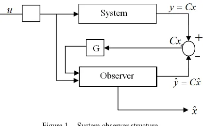
In the sensorless speed control of induction motors with direct field orientation [6], the rotor flux and speed information are dependent on the observers. However, the exact values of the parameters that construct the observers are difficult to measure and changeable with respect to the operating conditions. When the motor parameters are changed and thus different from the preset values, the estimated flux will deviate from the real values. To make flux estimation robust to parameter variations, a flux observer is proposed in the paper. System observer structure is shown in Fig. 1. The stability of the method is proven by Lyapunov theory.
Figure 1. System observer structure.
The speed
x
1a is taken as ‘constant’. Then the last four equations of (1) can be written in steady space form as,Cx
y
Bu
Ax
x
(2)Here we have,
9 7 1 8 9 1 8 7 6 5 1 6 1 5 0 ) ( 0 ) ( a a x a a x a a a a x a x a A a a a a a a a a (3)
Input matrix B,
b b B 0 0 0 0 0 0
and output matrix,
1 0 0 0 0 1 0 0 C
C. Flux Observer Design
Let the flux is not measured. The stator current and speed both are measurable. And also consider that the speed
x
1
r, and then these equations are rewritten in the following,
5 6 3 5 2 3 4 6 3 2 5 2)
(
)
(
x
a
x
a
x
x
x
a
x
x
a
x
r a r a
(4)Let estimated dynamics of (3.3) be,
5 6 3 5 2 1 3 4 6 3 1 2 5 2 ˆ ˆ ˆ ) ˆ ( ˆ ˆ ˆ ) ˆ ( ˆ ˆ x a x a x x x x a x x x a x a a a a (5)
The error dynamics is obtained by substituting (5) from (4), to give,
e a r e e a r e e a r e a r e e x a x x x a x x x a x x x x a x 5 6 2 1 3 5 2 3 4 6 3 1 3 2 5 2 ˆ ) ˆ ( ) ( ˆ ) ˆ ( ) ( (6)
2 5 9 4 3 7 2 1 8 5 1 5 4 9 3 1 8 2 7 4 5 6 3 5 2 1 3 4 6 3 1 2 5 2 ˆ ˆ ˆ ˆ ˆ ˆ ˆ ˆ ˆ ˆ ˆ ˆ ˆ ˆ ˆ ) ˆ ( ˆ ˆ ˆ ) ˆ ( ˆ ˆ bu x a x x a x x a x bu x x a x x a x a x x a x a x x x x a x x x a x a a a a a a a a
(7)Subtracting (1) from (7) gives,
e e a e e a e e e a e e a e e e e a r e e a r e e a r e a r e e x a x x a x x a x x a x x x a x x a x a x x a x x a x x x a x x x a x x x x a x 5 9 4 3 7 2 1 8 1 2 8 5 5 4 9 3 1 8 2 7 1 3 8 4 5 6 2 1 3 5 2 3 4 6 3 1 3 2 5 2 ˆ ˆ ˆ ) ˆ ( ) ( ˆ ) ˆ ( ) (
(8)With estimations the equation (2) becomes,
Bu
x
A
x
ˆ
ˆ
(9)Subtracting (9) from (2) gives,
x
A
Ax
x
x
x
e
ˆ
e
ˆ
ˆ
(10)And
e e e e ex
x
x
x
x
5 4 3 2 (11)Let the observer equation be shown by,
o
Gu Bu x A
xˆ ˆˆ (12)
In (12) the observer input is given by
u
o along withthe observer input matrix G[7]. Then subtracting (12)
from (2) shall lead to the same equation (10) with
Gu
oas additional term on the right hand side, and
u
o
Cx
e. Then (12) can be rewritten as,e
GCx
Bu
x
A
x
ˆ
ˆ
ˆ
(13)Subtracting (13) from (2), then the estimation error dynamics becomes,
(
)
e e e
e e
x
Ax
GCx
x
A GC x
(14)To minimize the estimation error let the Lyapunov function [8] be chosen as,
e T e
x
x
V
(15)Then for asymptotic stability and convergence the
time derivative of
V
must be negative semi-definite or,e T e e T
e
x
x
x
x
V
(16)Substituting (14) into (16) with
e
o Cx
u shall give,
e T e e T T T T
e A C G x x A CG x
x
V ( ) ( )
e T
T
e A GC A GC x
x
V {( ) ( )} (17)
For stability
V
0
it is required to have,0 )
(AGC
i.e. is eigen values should have negative real parts. So G is chosen in such a manner that
)
(AGC has the eigen values in negative real part.
III. SIMULATION AND RESULTS
In this paper, the state dynamics of induction machine with observer is simulated. Simulation models and results are explained. And conclusion from results is discussed at last of paper.
The rating and parameter of three phase induction motor taken for simulation are given in Table I [9]. In this work, Matlab 7.3 simulink is used to simulate the state dynamics of motor with observer.
TABLE I. PARAMETERS OF INDUCTION MOTOR.
S.
N. Parameters of induction motor Value
1. Stator resistance 0.262
2. Rotor resistance 0.187
3. Stator inductive reactance 1.206
4. Rotor inductive reactance 1.206
5. Mutual inductance 547.02
6. Number of poles 4
7. Moment of inertia of motor and load 2
06 . 11 kg m
J
The various coefficient of induction motor dynamic is given by, 4 . 164 , 06 . 68 ) ( , 3932 . 0 26 . 2 , 57 . 63 , 747 . 5 , 0006488 . 0 4 3 2 2 9 8 6 7 6 5 1 D X b X r X r X D a D X a D a a rr X X r a rr X r a X X J P a rr b M r rr s rr b M M r b r b b rr M
J k a J k J f a J k
a 2
4 1 3
0
2 , ,
Here,
k
0,
k
1&k
2denotes inertia load, friction and fan load coefficient respectively, where,k
2
k
1
k
0 A. Under No LoadThe simulation results under no load conditions are shown in Fig. 2 and Fig. 3. Fig. 2 shows observed quadrature axis rotor flux and Fig. 3 shows observed direct axis rotor flux.And Fig. 3 and Fig. 4 are showing the error in quadrature axis rotor flux estimation under no load and direct axis rotor flux estimation under no load respectively.
Figure 2. Observed quadrature axis rotor flux under no load condition.
Figure 3. Observed direct axis rotor flux under no load condition.
Figure 4. Error in quadrature axis rotor flux estimation under no load.
Figure 5. Error in direct axis rotor flux estimation under no load.
B. Under Load
Figure 6. Observed quadrature axis rotor flux under load condition.
Figure 7. Observed direct axis rotor flux under load condition.
Figure 8. Error in quadrature axis rotor flux estimation under load.
0 1 2 3 4 5 6
-800 -600 -400 -200 0 200 400 600
Q
u
a
d
ra
tu
re
a
x
is
r
o
to
r
fl
u
x
(
b)
Time (second)
0 1 2 3 4 5 6
-1000 -500 0 500 1000 1500 2000
D
ire
ct
a
xi
s
ro
to
r
flu
x
(
b)
Time (second)
0 1 2 3 4 5 6
-2.5 -2 -1.5 -1 -0.5 0 0.5 1 1.5 2
2.5x 10
-12
E
rr
o
r
in
q
u
a
d
ra
tu
re
a
x
is
r
o
to
r
fl
u
x
(
b)
Time (second)
0 1 2 3 4 5 6
-2.5 -2 -1.5 -1 -0.5 0 0.5 1 1.5 2 2.5x 10
-12
E
rr
or
in
d
ire
ct
a
xi
s
ro
to
r
flu
x
(
b)
Time (second)
0 1 2 3 4 5 6
-800 -600 -400 -200 0 200 400 600
Q
ua
dr
at
ur
e
ax
is
r
ot
or
f
lu
x
(
b)
Time (second)
0 1 2 3 4 5 6
-1000 -500 0 500 1000 1500 2000
D
ire
ct
a
xi
s
ro
to
r f
lu
x
(
b)
Time (second)
0 1 2 3 4 5 6
-2.5 -2 -1.5 -1 -0.5 0 0.5 1 1.5 2
2.5x 10
-12
E
rr
or
in
q
ua
dr
at
ur
e
ax
is
r
ot
or
f
lu
x
(
b)
Figure 9. Error in direct axis rotor flux estimation under load.
The simulation results under load condition (Load: step (amplitude 1980) at t = 4 second.) are shown in Fig. 6 and Fig. 7. Fig. 6 shows observed quadrature axis rotor flux and Fig. 7 shows observed direct axis rotor flux.And Fig. 8 and Fig. 9 are showing the error in quadrature axis rotor flux estimation under load and direct axis rotor flux estimation under load respectively.
IV. CONCLUSION
This paper has presented a new approach for estimating a rotor flux based on the adaptive control theory. This approach can lead to a direct field oriented induction motor control without speed sensors. The influence of the parameter variation on the flux estimation can be removed by the proposed parameter adaptive scheme. The validity of the adaptive flux observer has been verified using simulation.
REFERENCES
[1] G. Ellis, Observers in Control System, Academic Press, 2002.
[2] Hisao, Kouki, and Nakano, “DSP-based speed adaptive flux observer of induction motor,” IEEE Transactions on Industry Applications, vol. 29, no. 2, March-April 1993.
[3] P. Vas, Sensorless Vector and Direct Torque Control, New York: Oxford University Press, 1998.
[4] H. W. Kim and S. K. Sul, “A new motor speed estimator using Kalman filter in low speed range,” IEEE Tran. Industrial Electronics, vol. 43, no. 4, pp. 498-504, Aug. 1996.
[5] G. C. Verghese and S. R. Sanders, “Observers for flux estimation in the induction machine,” IEEE Tran. Industrial Electronics, vol. 35, no. 1, pp. 85-94, 1998.
[6] P. L. Jansen and R. D. Lorenz “Observer based direct field orientation: Analysis and comparison of alternative methods,”
IEEE Tran. Industry Application, vol. 30, no. 4, pp. 945-953, 1994.
[7] Robyns and Frederique, “A methodology to determine gains of induction motor flux observers based on a theoretical parameter sensitivity analysis,” IEEE Tran. Power Electronics, vol. 15, no. 6, pp. 983-995, 2000.
[8] M. Krstic, I. Kanellakopoulos, and P. Kokotovic, Nonlinearand Adaptive Control System, John Wiley and Sons, 1995.
[9] P. C. Krause, Analysis of Electrical Machine, McGraw-Hill, New York, 1986.
Sharad Salunke received the M.E. degree. in
Electrical Engineering with specialization in digital techniques & instrumentation in 2010 from SGSITS, Indore, M.P., India. He is currently working as an Assistant Professor in Sagar Institute of Research & Technology, Bhopal, M.P., India. He also worked as Head of the Department of Electrical & Electronics Engineering at Vikrant Institute of Technology & Management, Indore, M.P., India. His research interests include Nonlinear Control Systems, Digital Image Processing. and A.C. machines. This author became an Associate Member (AM) of IE in 2012.
Ashish Sharma received the M.E. degree. in
Electrical Engineering with specialization in digital techniques & instrumentation in 2010 from SGSITS, Indore, M.P., India. He is currently working as an Assistant Professor in SGSITS, Indore, M.P., India. His research interests include Nonlinear Control Systems, Digital Signal Processing and Digital Image Processing.
0 1 2 3 4 5 6
-2.5 -2 -1.5 -1 -0.5 0 0.5 1 1.5 2
2.5x 10
-12
E
rr
or
in
d
ire
ct
a
xi
s
ro
to
r
flu
x
(
b)