Relaxed Marginal Inference and its Application to Dependency Parsing
Sebastian Riedel David A. Smith Department of Computer Science University of Massachusetts, Amherst
{riedel,dasmith}@cs.umass.edu
Abstract
Recently, relaxation approaches have been successfully used for MAP inference on NLP problems. In this work we show how to extend the relaxation approach to marginal inference used in conditional likelihood training, pos-terior decoding, confidence estimation, and other tasks. We evaluate our approach for the case of second-order dependency parsing and observe a tenfold increase in parsing speed, with no loss in accuracy, by performing in-ference over a small subset of the full factor graph. We also contribute a bound on the error of the marginal probabilities by a sub-graph with respect to the full graph. Finally, while only evaluated with BP in this paper, our ap-proach is general enough to be applied with any marginal inference method in the inner loop.
1 Introduction
In statistical natural language processing (NLP) we are often concerned with finding the marginal proba-bilities of events in our models or the expectations of features. When training to optimize conditional like-lihood, feature expectations are needed to calculate the gradient. Marginalization also allows a statis-tical NLP component to give confidence values for its predictions or to marginalize out latent variables. Finally, given the marginal probabilities of variables, we can pick the values that maximize these marginal probabilities (perhaps subject to hard constraints) in order to predict a good variable assignment.1
1With a loss function that decomposes on the variables, this
amounts to Minimum Bayes Risk (MBR) decoding, which is
Traditionally, marginal inference in NLP has been performed via dynamic programming (DP); how-ever, because this requires the model to factor in a way that lends itself to DP algorithms, we have to restrict the class of probabilistic models we con-sider. For example, since we cannot derive a dy-namic program for marginal inference in second or-der non-projective dependency parsing (McDonald and Satta, 2007), we have non-projective languages such as Dutch using second order projective mod-els if we want to apply DP. Some previous work has circumvented this problem for MAP inference by starting with a second-order projective solution and then greedily flipping edges to find a better non-projective solution (McDonald and Pereira, 2006).
In order to explore richer model structures, the NLP community has recently started to investigate the use of other, well-known machine learning tech-niques for marginal inference. One such technique is Markov chain Monte Carlo, and in particular Gibbs sampling (Finkel et al., 2005), another is (loopy) sum-product belief propagation (Smith and Eisner, 2008). In both cases we usually work in the frame-work of graphical models—in our case, with factor graphs that describe our distributions through vari-ables, factors, and factor potentials. In theory, meth-ods such as belief propagation can take any graph and perform marginal inference. This means that we gain a great amount of flexibility to represent more global and joint distributions for NLP tasks.
The graphical models of interest, however, are often too large and densely connected for efficient inference in them. For example, in second order
often very effective.
dependency parsing models, we have O(n2) vari-ables and O(n3) factors, each of which may have
to be inspected several times. While belief prop-agation is still tractable here (assuming we follow the approach of Smith and Eisner (2008) to enforce tree constraints), it is still much slower than sim-pler greedy parsing methods, and the advantage sec-ond order models give in accuracy is often not sig-nificant enough to offset the lack of speed in prac-tice. Moreover, if we extend such parsing models to, say, penalizing all pairs of crossing edges or scoring syntax-based alignments, we will need to inspect at leastO n4 factors, increasing our efficiency con-cerns.
When looking at the related task of finding the most likely assignment in large graphical models (i.e., MAP inference), we notice that several recent approaches have significantly sped up computation through relaxation methods (Tromble and Eisner, 2006; Riedel and Clarke, 2006). Here we start with a small subset of the full graph, and run inference for this simpler problem. Then we search for factors that are “violated” in the solution, and add them to the graph. This is repeated until no more new factors can be added. Empirically this approach has shown impressive success. It often dramatically reduces the effective network size, with no loss in accuracy.
How can we extend or generalize MAP relax-ation algorithms to the case of marginal inference? Roughly speaking, we answer it by introducing a notion of factor gain that is defined as the KL di-vergence between the current distribution with and without the given factor. This quantity is then used in an algorithm that starts with a sub-model, runs marginal inference in it and then determines the gains of the not-yet-added factors. In turn, all fac-tors for which the gain exceeds some threshold are added to the current model. This process is repeated until no more new factors can be found or a maxi-mum number of iterations is reached.
We evaluate this form ofrelaxed marginal infer-encefor the case of second-order dependency pars-ing. We follow Smith and Eisner’s tree-aware be-lief propagation procedure for inference in the inner loop of our algorithm. This leads to a tenfold in-crease in parsing speed with no loss in accuracy.
We also contribute a bound on the error on marginal probabilities the sub-graph defines with
re-spect to the full graph. This bound can be used both for terminating (although not done here) and under-standing the dynamics of inference. Finally, while only evaluated with BP so far, it is general enough to be applied with any marginal inference method in the inner loop.
In the following, we first give a sketch of the graphical model we apply. Then we briefly discuss marginal inference. In turn we describe our relax-ation algorithm for marginal inference and some of its theoretic guarantees. Then we present empirical support for the effectiveness of our approach, and conclude.
2 Graphical Models of Dependency Trees
We give a brief overview of the graphical model we apply in our experiments. We chose the grandpar-ents and siblings model, together with language spe-cific multiroot and projectivity options as taken from Smith and Eisner (2008). All our models are defined over a set of binary variablesLij that indicate a
de-pendency between tokeni and j of the input sen-tenceW.
2.1 Markov Random Fields
Following Smith and Eisner (2008), we define a probability distribution over all dependency trees as a collection of edges y for a fixed input sentence
W. This distribution is represented by an undirected graphical model, or Markov random field (MRF):
pF(y)def=
1
Z Y
i∈F
Ψi(y) (1)
specified by an index set F and a corresponding family(Ψi)F offactors Ψi : Y 7→ <+. Here Z
is the partition functionZF =PyQiΨi(y).
We will restrict our attention to binary factors that can be represented asΨi(y) =eθiφi(y)with binary
functionsφi(y)∈ {0,1}and weightsθi ∈ <.2 This
2
Theseφiare also calledsufficient statisticsorfeature
leads to
pF(y)def=
1
Z exp X
i∈F
θiφi(y)
!
as an alternative representation for pF. Note that
whenφi(y) = 1we will say thatΨifiresfory.
Note that a factor function Ψi(y) can depend on
any part of the observed input sentenceW; however, for brevity we will suppress this extra argument to Ψi.
2.2 Hard and Soft Constraints on Trees
A particular model specifies its preference for set of dependency edges over another by a set of hard and soft constraints. We use hard constraints to rule out
a prioriillegal structures, such as trees where a word has two parents, and soft constraints to raise or lower the score of trees that contain particular good or bad substructures.
Ahardfactor (or constraint)Ψi evaluates an
as-signment y with respect to some specified condi-tion and fires only if this condicondi-tion is violated; in this case it evaluates to 0. It is therefore ruling out all configurations in which the condition does not hold. Note that a hard constraintΨi corresponds to
θi=−∞in our loglinear representation.
For dependency parsing, we consider two partic-ular hard constraints, each of which touches all edge variables iny: the constraintTree requires that all edges form a directed spanning tree rooted at the root node 0; the constraintPTreeenforces the more stringent condition that all edges form a projective
directed tree. As in (Smith and Eisner, 2008), we used algorithms from edge-factored parsing to com-pute BP messages for these factors. In our experi-ments, we enforced one or the other constraint de-pending on the projectivity of given treebank data.
A soft factor Ψi acts as a soft constraint that
prefers some assignments to others. This is equiv-alent to saying that its weightθi is finite. Note that
the weight of a soft factor is usually itself composed as a sum of (sub-)weights wj for feature functions
that have the same input-output behavior as φi(y)
when conditioned on the current sentence. It is these
wjwhich are adjusted at training time.
We use three kinds of soft factors from Smith and Eisner (2008). In the full model, there are: O(n2)
LINKi,j factors that judge dependency edges in
iso-lation; O(n3) GRAND
i,j,k factors that judge pairs
of dependency edges in a grandparent-parent-child chain; andO(n3)SIBi,j,kfactors that judge pairs of
dependency edges that share the same parent.
3 Marginal Inference
Formally, given our set of factorsFand an observed sentence W, marginal inference amounts to calcu-lating the probabilityµFi that our binary featuresφi
are active. That is, for each factorΨi
µFi def= X
φi(y)=1
pF(y) =EF[φi] (2)
For compactness, we follow the convention of Wain-wright and Jordan (2008) and represent the belief for a variable using the marginal probability of its cor-responding unary factor. Hence, if we want to calcu-latepF(Lij)we useµFLINKijin place. Moreover we
will useµF¬i def= 1−µFi when we need the probability of the eventφi(y) = 0.
The two most prominent approaches to marginal inference in general graphical models are Markov Chain Monte Carlo (MCMC) and variational meth-ods. In a nutshell, MCMC iteratively generates a Markov chain that yieldspF as its stationary
distri-bution. Any expectationµFi can then be calculated simply by counting the corresponding statistics in the generated chain.
Generally speaking, variational methods frame marginal inference as an optimization problem. Ei-ther in the sense of minimizing the KL divergence of a much simpler distribution to the actual distribu-tionpF, as in mean field methods. Or in the sense of
maximizing a variational representation of the log-partition function over the setMofvalidmean vec-tors (Wainwright and Jordan, 2008). Note that the variational representation of the log partition func-tion involves an entropy term that is intractable to calculate in general and therefore usually approxi-mated. Likewise, the set of constraints that guaran-tee vectorsµto be valid mean vectors is intractably large and is often simplified.
uses the Bethe Free Energy as approximation to the entropy, and the setMLof locally consistent mean vectors as an outer bound onM. A mean vector is locally consistent if its beliefs on factors are consis-tent with the beliefs of the factor neighbors.
BP solves the variational problem by iteratively updating the beliefs of factors and variables based on the current beliefs of their neighbors. When ap-plied to acyclic graphical models BP yields the exact marginals at convergence. For general graphs, BP is not guaranteed to converge, and the beliefs it calcu-lates are generally not the true marginals; however, in practice BP often does converge and lead to accu-rate marginals.
4 Relaxed Incremental Marginal Inference
Generally the runtime and accuracy of a marginal in-ference method depends on size, density, tree-width and interaction strength (i.e. the magnitude of its weights) of the Graphical Model. For example, in Belief Propagation the number of messages we have to send in each iteration scales with the number of factors (and their degrees). This means that when we add a large number of extra factors to our model, such as the O(n3) grandparent and sibling factors for dependency parsing, we have to pay a price in terms of speed, sometimes even accuracy.
However, on close inspection often many of the additional factors we use to model some higher or-der interactions are somewhat unnecessary or redun-dant. To illustrate this, let us look at a second or-der parsing model with grandparent factors. Surely determiners are not heads of other determiners, and this should be easy to encourage using LINK fea-tures only. Hence, a grandparent factor that dis-courages a determiner-determiner-determiner chain seems unnecessary.
This raises two questions: (a) can we get away without most of these factors, and (b) can we effi-ciently tell which factors should be discarded. We will see in section 5 that question (a) can be an-swered affirmatively: with a only fraction of all sec-ond order factors we can calculate marginals that are very close to the BP marginals, and when used in MBR decoding, lead to the same trees.
Question (b) can be approached by looking at how a similar problem has been tackled in
combinato-rial optimization and MAP inference. Riedel and Clarke (2006) tackled the MAP problem for depen-dency parsing by an incremental approach that starts with a relaxation of the problem, solves it, and adds additional constraints only if they are violated. If constraints were added, the process is repeated, oth-erwise we terminate.
4.1 Evaluating Candidate Factors
To develop such an incremental relaxation approach to marginal inference, we generalize the notion of a violated constraint. What does it mean for a factor to be violated with respect to the solution of a marginal inference problem?
One answer is to interpret the violation of a con-straint as “adding this concon-straint will impact our cur-rent belief”. To assess the impact of adding factor Ψito a sub-graphF0 ⊆ F we can then use the
fol-lowing intuition: if the distributionF0∪ {i}is very similar to the distribution corresponding toF0, it is
probably safe to say that the marginals we get from both are close, too. If we use the KL divergence be-tween the (distributions of)F0∪ {i}andF0 for our
interpretation of the above mentioned closeness, we can define a potentialgainfor addingΨias follows:
gF0(Ψi)def= DKL pF0||pF0∪{i}.
Together with a threshold on this gain we can now adapt the relaxation approach to marginal in-ference by simply replacing the question, “IsΨi
vi-olated?” with the question, “IsgF0(i) > ?” We
can see the latter question as a generalization of the former if we interpret MAP inference as the zero-temperature limit of marginal inference (Wainwright and Jordan, 2008).
The form of the gain function is chosen to be eas-ily evaluated using the beliefs we have already avail-able for the current sub-graphF0. It is easy to show (see Appendix) that the following holds:
Proposition 1. The gain of a factorΨiwith respect
to the sub-graphF0 ⊆ F is
gF0(Ψi) = log
µF¬i0 +µF
0
i eθi
−µFi 0θi (3)
That is, the gain of a factor Ψi depends on two
properties of Ψi. First, the expectation µF
0
i that
its loglinear weight θi. To get an intuition for this
gain, consider the limitlimµF 0 i →1
gF0(Ψi)of a
fac-tor with positive weight that is expected to be active underF0. In this case the gain becomes zero,
mean-ing that the more likely Ψi fires under the current
model, the less useful will it be to add according to our gain. ForlimµF 0
i →0gF
0(Ψi)the gain also
disap-pears. Here the confidence of the current model inφi
being inactive is so high that any single factor which indicates the opposite cannot make a difference.
Fortunately, the marginal probability µFi 0 is usu-ally available after inference, or can be approxi-mated. This allows us to maintain the same basic algorithm as in the MAP case: in each “inspection step” we can use the results of the last run of infer-ence in order to evaluate whether a factor has to be added or not.
4.2 Algorithm
Algorithm 1 shows our proposed algorithm,Relaxed Marginal Inference. We are given an initial factor graph (for example, the first order dependency pars-ing model), a thresholdon the minimal gain a fac-tor needs to have in order to be added, and a solverS
for marginal inference in the partial graphs we gen-erate along the way.
We start by finding the marginalsµfor the initial graph. These marginals are then used in step 4 to find the factors that would, when added in isolation, change the distribution substantially (i.e., by more than in terms of KL divergence). We will refer to this step asseparation, in line with cutting plane terminology. The factors are added to the current graph, and we start from the top unless there were no new factors added. In this case we return the last marginalsµ.
Clearly, this algorithm is guaranteed to converge: either we add at least one factor per iteration until we reach the full graph F, or we converge before. However, it is difficult to make any general state-ments about the number of iterations it takes until convergence. Nevertheless, in our experiments we find that algorithm 1 converges to a much smaller graph after a small number of iterations, and hence we are always faster than inference on the full graph. Finally, note that calculating the gain for all fac-tors inF \ F0 in step 4 (separation) takes time
pro-Algorithm 1Relaxed Marginal Inference.
1: require:
F0
:init. graph,:threshold,S:solver,R:max. it 2: repeat
Find current marginals using solver S
3: µ←marginals(F0, S)
Find factors with high gain not yet added
4: ∆F ← {i∈ F \ F0|gF0(Ψi)> }
Add factors to current graph
5: F0 ← F0∪∆F
Check: no more new factors were added or R reached
6: until∆F=∅or iteration >R
return the marginals for the last graphF0
7: returnµ
portional to|F \ F0|.
4.3 Accuracy
We have seen how to evaluate the potential gain when adding a single factor. However, this does not tell us how good the current sub-model is with respect to the complete graph. After all, while all remaining factors individually might not contribute much, in concert they may. We therefore present a (calculable) bound on the KL divergence of the par-tial graph from the full graph that can give us confi-dence in the solutions we return at convergence.
Note that for this bound we still only need fea-ture expectations from the current model. More-over, we assume all weightsθiare positive—without
loss of generality since we can always replace φi
with its negation 1−φi and then change the sign
ofθi(Richardson and Domingos, 2006).
Proposition 2. Assume non-negative weights, let
F0 ⊆ F be a subset of factors, G def= F \ F0 and
ηdef=kθGk1− hµG, θGi ≥0. Then
1. for the KL divergence betweenF0 and the full
networkF we have:
DKL pF0||pF
≤η.
2. for the error we make when estimatingφi’s true
expectationµFi byµFi 0 we have:
−(eη−1)µF¬i0 ≤µ
F
i −µ
F0
i ≤(eη −1)µ
F0
This says that (1) we get closer to the full distri-bution and that (2) our marginals closer to the true marginals, if the remaining factors G either have a low total weight kθGk, or the current belief µG
already assigns high probability to the features φG
being active (and hence− hµG, θGi is small). The
latter condition is the probabilistic analog to con-straints already being satisfied. Finally, sinceηcan be easily calculated, we plan to investigate its utility as a convergence criterion in future work.
4.4 Related Work
Our approach is inspired by earlier work on re-laxation algorithms for performing MAP inference by incrementally tightening relaxations of a graph-ical model (Anguelov et al., 2004; Riedel, 2008), weighted Finite State Machine (Tromble and Eisner, 2006), Integer Linear Program (Riedel and Clarke, 2006) or Marginal Polytope (Sontag et al., 2008). However, none of these methods apply to marginal inference.
Sontag and Jaakkola (2007) compute marginal probabilities by using a cutting plane approach that starts with the local polytope and then optimizes some approximation of the log partition function. Cycle consistency constraints are added if they are violated by the current marginals, and the process is repeated until no more violations appear. While this approach does tackle marginalization, it is focused on improving its accuracy. In particular, the opti-mization problems they solve in each iteration are in fact larger than the problem we want to relax.
Our approach is also related to edge deletion in Bayesian networks (Choi and Darwiche, 2006). Here edges are removed from a Bayesian network in order to find a close approximation to the full net-work useful for other inference-related tasks (such as combined marginal and MAP inference). The core difference to our approach is the fact that they ask which edges to removefrom the full graph, in-stead of which to add to a partial graph. This re-quires inference in the full model—the very opera-tion we want to avoid.
5 Experiments
In our experiments we seek to answer the following questions. First, how fast is our relaxation approach
compared to full marginal inference at comparable dependency accuracy? This requires us to find the best tree in terms of marginal probabilities on the link variables (Smith and Eisner, 2008). Second, how good is the final relaxed graph as an approxima-tion of the full graph? Finally, how does incremental relaxation scale with sentence length?
5.1 Data and Models
We trained and tested on a subset of languages from the CoNLL Dependency Parsing Shared Tasks (Nivre et al., 2007): Dutch, Danish, Italian, and English. We apply non-projective second order models for Dutch, Danish and Italian, and a projec-tive second order model for English. To be able to compare inference on the same model, we trained using BP on the full set of LINK, GRAND, and SIB factors.
Note that our models would rank highly among the shared task submissions, but could surely be fur-ther improved. For example, we do not use any lan-guage specific features. Since our focus in this paper is speeding up marginal inference, we will search for better models in future work.
5.2 Runtime and Dependency Accuracy
In our first set of experiments we explore the speed and accuracy of relaxed BP in comparison to full BP. To this end we first tested BP configurations with at most 5, at most 10, and at most 50 iterations to find the best setup in terms of speed and accuracy. Smith and Eisner (2008) use 5 iterations but we found that by using 10 iterations accuracy could be slightly im-proved. Running at most 50 iterations led to the same accuracy but was significantly slower. Hence we only report BP results with 10 iterations here.
For relaxed BP we tested along three dimensions: the thresholdon the gain of factors, the maximum number of BP iterations in the inner loop of relaxed BP, and the maximum number of relaxation itera-tions. A configuration with maximum relaxation it-erationsR, threshold, and maximum BP iterations
B will be identified by RelR,,B. In all settings we
use the LINKfactors and the hard factors as initial graphF0.
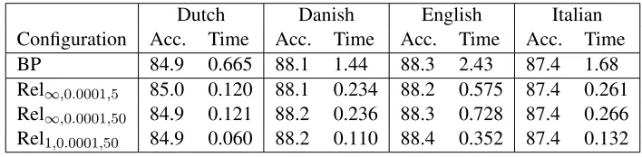
iden-Dutch Danish English Italian Configuration Acc. Time Acc. Time Acc. Time Acc. Time BP 84.9 0.665 88.1 1.44 88.3 2.43 87.4 1.68 Rel∞,0.0001,5 85.0 0.120 88.1 0.234 88.2 0.575 87.4 0.261
Rel∞,0.0001,50 84.9 0.121 88.2 0.236 88.3 0.728 87.4 0.266
[image:7.612.128.482.59.146.2]Rel1,0.0001,50 84.9 0.060 88.2 0.110 88.4 0.352 87.4 0.132
Table 1: Dependency accuracy (%) and average parsing time (sec.) using second order models.
tified heads) in comparison to the gold data, and av-erage parsing time in seconds. Here parsing time includes both time spent for marginal inference and the MBR decoding step after the marginals are avail-able.
We notice that by relaxing BP with no limit on the number of iterations we gain a 4-6 fold increase in parsing speed across all languages when using the threshold = 0.0001, while accuracy remains as high as for full BP. This can be achieved with fewer BP iterations (at most 5) in each round of relaxation than full BP needs per sentence (at most 10). Intu-itively this makes sense: since our factor graphs are smaller in each iteration there will be fewer cycles to slow down convergence. This only has a small impact on overall parsing time for languages other than English, since for most sentences even full BP converges after less than 10 iterations.
We also observe that running just one iteration of our relaxation algorithm (Rel1,0.0001,50) is enough to
achieve accurate solutions. This leads to a twofold speed-up in comparison to running relaxation until convergence (primarily because of fewer calls to the separation routine), and a 7-13 fold speed-up (ten-fold on average) when compared to full BP.
5.3 Quality of Relaxed Subgraphs
How large is the fraction of the full graph needed for accurate marginal probabilities? And do we re-ally need our relaxation algorithm with repeated in-ference or could we instead just prune the graph in advance? Here we try to answer these questions, and will focus on the Danish dataset. Note that our re-sults for the other languages follow the same pattern. In table 2, we present the average ratio of the sizes of the partial and the full graph in terms of the sec-ond order factors. We also show the total runtime needed to find the subgraph and run inference in it.
Configuration Size Time Err. Acc.
BP 100% 1.44 — 88.1
Rel∞,0.1,50 ≈0% 0.12 0.20 87.5
Rel∞,0.0001,50 0.8% 0.24 0.012 88.2
Rel1,0.0001,50 0.8% 0.11 0.015 88.2
Pruned0.1 42% 0.56 0.022 88.0
Pruned0.5 22% 0.40 0.098 87.7
Table 2: Ratio of partial and full graph size (Size), runtime in seconds (Time), avg. error on marginals (Err.) and tree accuracy (Acc.) for Danish.
As a measure of accuracy for marginal probabilities we find the average error in marginal probability for the variables of a sentence. Note that this measure does not necessarily correspond to the true error of our marginals because BP itself is approximate and may not return the correct marginals.
The first row shows the full BP system, working on 100% of the factor graph. The next three rows look at relaxed marginal inference. We notice that with a low threshold= 0.1we pick almost no ad-ditional factors (0.003%), and this does affect accu-racy. However, by lowering the threshold to 0.0001 and adding about 0.8% of the second order factors, we already match the dependency accuracy of full BP. On average we are also very close to the BP marginals.
Can we find such small graphs without running extra iterations of inference? One approach could be to simply cut off factorsΨiwith absolute weights
|θi|that fall under a certain thresholdt. In the final
rows of the table we test such an approach witht= 0.1,0.5.
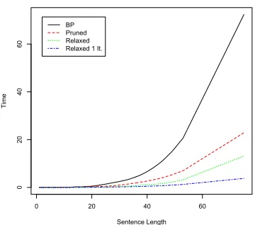
0 20 40 60
0
20
40
60
Sentence Length
T
ime
BP Pruned
Relaxed
[image:8.612.91.271.78.237.2]Relaxed 1 It.
Figure 1: Total runtimes by sentence length.
size further to about 20%, accuracy drops below the values we achieved with our relaxation approach at 0.8% of the second order factors. Hence simple pruning removes factors that do have a low weight, but are still important to keep.
5.4 Runtime with Varying Sentence Length
We have seen how relaxed BP is faster than full BP on average. But how does its speed scale with sentence length? To answer this question figure 1 shows a plot of runtime by sentence length for full BP, pruned BP with threshold0.1, Rel∞,0.0001,50and
Rel1,0.0001,50.
The graph indicates that the advantage of relaxed BP over both full BP and Pruned BP becomes even more significant for longer sentences, in particular when running only one iteration. This shows that by using our technique, second order parsing becomes more practical, in particular for very long sentences.
6 Conclusion
We have presented a novel incremental relaxation al-gorithm that can be applied to marginal inference. Instead of adding violated constraints in each iter-ation, it adds factors that significantly change the distribution of the graph. This notion is formalized by the introduction of a gain function that calculates the KL divergence between the current network with and without the candidate factor. We show how this gain can be calculated and provide bounds on the
er-ror made by the marginals of the relaxed graph in place of the full one.
Our algorithm led to a tenfold reduction in run-time at comparable accuracy when applied to multi-lingual dependency parsing with Belief Propagation. It is five times faster than pruning factors by their absolute weight, and results in smaller graphs with better marginals.
In future work we plan to apply relaxed marginal inference to larger joint inference problems within NLP, and test its effectiveness with other marginal inference algorithms as solvers in the inner loop.
Acknowledgments
This work was supported in part by the Center for Intelligent Information Retrieval and in part by SRI International subcontract #27-001338 and ARFL prime contract #FA8750-09-C-0181. Any opinions, findings and conclusions or recommendations ex-pressed in this material are the authors’ and do not necessarily reflect those of the sponsor.
Appendix: Proof Sketches
For Proposition 1 we use the primal form of the KL diver-gence (Wainwright and Jordan, 2008)
D`
p0F||pF´= log`ZFZF−01 ´
− hµF0, θF−θF0i
and represent the ratioZFZF−01of partition functions as
ZF
ZF0
=X
y
ehθF 0,φF 0(y)i ZF0
ehθG,φG(y)i=E
F0 h
ehθG,φGii
whereGdef=F \ F0. WithG={i}we get the desired gain. For Proposition 2, part 1, we first pick a simple upper bound onZFZF−01 by replacing the expectation withe
kθGk1.
Insert-ing this into the primal form KL divergence leads to the given bound. For part 2 we representpFusingpF0
pF(y) =ZF0ZF−1ehθG,φG(y)ipF0(y)
and reuse our above representation ofZFZF−01. This gives
pF(y) =EF0 h
ehθG,φG(y)ii−1p
F0(y)ehθG,φG(y)i
which can be upper bounded by lower bounding the expectation and upper bounding the log-linear term. For the latter we use
ekθGk1, for the first Jensen’s inequality gives
EF0 h
ehθG,φG(y)ii
−1
≥eEF 0[hθG,φG(y)i]=e D
θG,µF 0G E
where the equality follows from linearity of expectations. This yieldspF(y)≤pF0(y)eηand therefore upper bounds onµFi
andµF¬i. Basic algebra then gives the desired error interval for
References
D. Anguelov, D. Koller, P. Srinivasan, S. Thrun, H.-C. Pang, and J. Davis. 2004. The correlated correspon-dence algorithm for unsupervised registration of non-rigid surfaces. In Advances in Neural Information
Processing Systems (NIPS ’04), pages 33–40.
Arthur Choi and Adnan Darwiche. 2006. A varia-tional approach for approximating bayesian networks by edge deletion. In Proceedings of the Proceedings of the Twenty-Second Conference Annual Conference on Uncertainty in Artificial Intelligence (UAI-06), Ar-lington, Virginia. AUAI Press.
Jenny Rose Finkel, Trond Grenager, and Christopher Manning. 2005. Incorporating non-local informa-tion into informainforma-tion extracinforma-tion systems by gibbs sam-pling. In Proceedings of the 43rd Annual Meeting of the Association for Computational Linguistics (ACL’ 05), pages 363–370, June.
R. McDonald and F. Pereira. 2006. Online learning of approximate dependency parsing algorithms. In
Proceedings of the 11th Conference of the European
Chapter of the ACL (EACL ’06), pages 81–88.
Ryan McDonald and Giorgio Satta. 2007. On the com-plexity of non-projective data-driven dependency
pars-ing. In IWPT ’07: Proceedings of the 10th
Inter-national Conference on Parsing Technologies, pages
121–132, Morristown, NJ, USA. Association for Com-putational Linguistics.
J. Nivre, J. Hall, S. Kubler, R. McDonald, J. Nilsson, S. Riedel, and D. Yuret. 2007. The conll 2007 shared task on dependency parsing. In Conference on Em-pirical Methods in Natural Language Processing and
Natural Language Learning, pages 915—932.
Matt Richardson and Pedro Domingos. 2006. Markov logic networks. Machine Learning, 62:107–136. Sebastian Riedel and James Clarke. 2006.
Incremen-tal integer linear programming for non-projective de-pendency parsing. InProceedings of the Conference on Empirical methods in natural language processing
(EMNLP ’06), pages 129–137.
Sebastian Riedel. 2008. Improving the accuracy and ef-ficiency of MAP inference for markov logic. In Pro-ceedings of the 24th Annual Conference on Uncer-tainty in AI (UAI ’08), pages 468–475.
David A. Smith and Jason Eisner. 2008. Dependency parsing by belief propagation. InProceedings of the Conference on Empirical Methods in Natural
Lan-guage Processing (EMNLP), pages 145–156,
Hon-olulu, October.
D. Sontag and T. Jaakkola. 2007. New outer bounds on the marginal polytope. InAdvances in Neural
Infor-mation Processing Systems (NIPS ’07), pages 1393–
1400.
David Sontag, T. Meltzer, A. Globerson, T. Jaakkola, and Y. Weiss. 2008. Tightening LP relaxations for MAP using message passing. InProceedings of the 24th An-nual Conference on Uncertainty in AI (UAI ’08). Roy W. Tromble and Jason Eisner. 2006. A fast
finite-state relaxation method for enforcing global con-straints on sequence decoding. In Joint Human Lan-guage Technology Conference/Annual Meeting of the North American Chapter of the Association for
Com-putational Linguistics (HLT-NAACL ’06), pages 423–
430.
Martin Wainwright and Michael Jordan. 2008. Graphi-cal Models, Exponential Families, and Variational