Simultaneous Detection and Fine Mapping of Quantitative Trait Loci
in Mice Using Heterogeneous Stocks
Richard Mott
1and Jonathan Flint
Wellcome Trust Centre for Human Genetics, Oxford University, Oxford, OX3 7BN, United Kingdom Manuscript received September 12, 2001
Accepted for publication January 28, 2002
ABSTRACT
We describe a method to simultaneously detect and fine map quantitative trait loci (QTL) that is especially suited to the mapping of modifier loci in mouse mutant models. The method exploits the high level of historical recombination present in a heterogeneous stock (HS), an outbred population of mice derived from known founder strains. The experimental design is an F2cross between the HS and a ge-netically distinct line, such as one carrying a knockout or transgene. QTL detection is performed by a standard genome scan withⵑ100 markers and fine mapping by typing the same animals using densely spaced markers over those candidate regions detected by the scan. The analysis uses an extension of the dynamic-programming technique employed previously to fine map QTL in HS mice. We show by simulation that a QTL accounting for 5% of the total variance can be detected and fine mapped with⬎50% probability to within 3 cM by genotypingⵑ1500 animals.
I
T is relatively straightforward to map quantitative trait without exhausting the resources of a single laboratory loci (QTL) that segregate in crosses between two and within a reasonable period of time (for instance, inbred strains, but identifying the responsible molecular within 3 years). One solution may be to use outbred variant is very taxing, largely because of the difficulties rather than inbred crosses, such as a genetically hetero-of resolving loci into intervals small enough to identify geneous stock (HS) derived from eight inbred strains genes (FlintandMott2001). Two general strategies and outbred for a number of generations prior to the have been adopted to fine map QTL. In the first, at- experiment (McClearnandMeredith1970). Histori-tempts are made to place a single QTL from one inbred cal recombination turns each HS chromosome into a strain on the genetic background of another. For exam- fine-grained mosaic of the founder strain haplotypes. ple, by breeding congenic mice derived from a cross of For example, after 60 generations (the current age of the two inbred strains used to detect the QTL, recombi- the HS animals we have used) the average distance nation can be used to reduce the size of the chromo- between recombinants is 1/60 or 1.7 cM. The large somal region containing the QTL. The second approach number of recombinants means that the HS can map exploits large numbers of recombinants across the ge- small to moderate effect QTL into subcentimorgan in-nome to fine map all QTL simultaneously. One way in tervals, as we have recently demonstrated (Talbot etwhich this can be done is by increasing the number of al.1999;McPeek2000;Mottet al.2000).
F2individuals in the cross used to detect the QTL. How- The HS has the potential to be a general-purpose tool
ever, for QTL with moderate or small effects, many for the genetic dissection of complex traits in model thousands of F2’s are needed to make the interval suffi- organisms, but it has a number of drawbacks. First,
ciently small to attempt positional cloning. This strategy whole genome scans using the HS require a very large is appropriate for species that are cheap to breed, such number of genotypes. To achieve power of 80% to de-as plants (AlpertandTanksley1996), but less suited tect a QTL accounting for 5% of the phenotypic vari-for livestock or laboratory rodents. In any event, the geno- ance, markers spacedⵑ1 cM apart across the whole ge-typing costs, which scale with the number of markers typed nome have to be genotyped on 2000 animals (Mott times the number of individuals, are almost prohibitive. et al. 2000). By contrast, for a similar QTL detection Alternatively, many generations of intercrossing may be experiment in an F
2cross, markers spaced every 20 cM
used to achieve subcentimorgan resolution (Darvasi and genotyped on a few hundred animals will suffice.
andSoller1995;Darvasi1997). Fewer genotypes are Second, the HS can be used only to fine map QTL that required, but the experiment takes much longer. segregate in crosses between the eight founder strains. Ideally we would like to map QTL to high resolution While this represents substantially more genetic
diver-sity than is found in most inbred crosses, it excludes the use of the HS for fine mapping many QTL of great 1Corresponding author:Wellcome Trust Centre for Human Genetics,
interest, for example, modifiers affecting mouse models
University of Oxford, Roosevelt Dr., Oxford, OX3 7AD, United
King-dom. E-mail: [email protected] of human disease.
A cross between an inbred and HS animal (which we call an inbred-outbred cross) extends the fine-mapping capacity of the HS, using F1 and F2 animals. Here we
develop and evaluate a particular type of inbred-outbred cross that requires data collected from the F2generation
only. The design is much like an F2intercross between
two inbred lines except that the data analysis means we can both detect and fine map QTL with high probability. The method makes it possible to screen the entire ge-nome of the HS with the same number of markers used in a backcross or F2 intercross and extends the use of
HS animals for fine mapping loci that modify the pheno-types produced by single-gene mutations (Threadgill et al.1995). The latter is of particular interest given the growing number of transgenic mice and the production of large numbers of novel mutants by random mutagen-esis (WellsandBrown2000).
Genetic mapping in HS populations is more complex
than mapping in inbred crosses, because at most marker Figure 1.—The inbred-outbred cross. An inbred line, I loci there are far fewer alleles than progenitor strains. (black chromosomes), is crossed with an outbred population, We find there are frequently only two or three alleles O. Each O chromosome is a fine-scale mosaic of known founder strains (represented as shaded segments). The F1
at a locus so that it is impossible to assign unambiguously
generation comprises homologous chromosomes that are
en-the strain of origin (of which en-there are eight) to each
tirelyIorO.The chromosomes from the F2generation contain
allele. The result is that single-marker association analy- a mixture ofIandOsegments. sis, the standard method for detecting QTL in inbred
crosses, cannot distinguish between strains having
dif-ferent QTL effects, but identical alleles, and therefore in the HS. The experimental design is an F2 cross
be-tween the outbred HS, denoted byO, and a background may fail to detect the QTL. We overcame this problem
using a multipoint analysis that uses a dynamic-program- line, I. For simplicity we assumeI is an inbred strain, although it is straightforward to extend the method so ming (DP) algorithm to assign the probability that an
allele descends from each progenitor in the HS. Under thatIis another outbred stock, provided it is genetically distinct from O.The F1 generation of theI ⫻O cross
an additive model of genetic action, the expected genetic
effect for a diploid individual with ancestral founders s comprises animals with homologous chromosomes that are either pureIorO.In the F2generation, formed by
andt at the QTL will be the sum of the strain effects
for these founders,Ts⫹Tt, say, of the QTL at the locus. crossing the F1’s with themselves, each chromosome will
contain roughly equal amounts of IandO with about A test for a QTL is then equivalent to testing for
differ-ences between strain effects by analysis of variance. Us- one recombinant per chromosome. The key point is that the F2 chromosomes contain Isegments with no
ing this approach we showed that in one experiment
single-marker association analysis detected only two out internal recombination and Osegments dense in re-combinants (Figure 1).
of five QTL detected by the DP method in the HS (Mott
et al.2000). The presence of two scales of recombination makes it possible to carry out low resolution QTL detection Analysis of the inbred-outbred cross must not only
assign progenitor strains to alleles in the HS, but addi- and high resolution QTL fine mapping in the same ani-mals. A single set of individuals from the F2generation
tionally it must confront the difficulty of distinguishing
alleles that descend from inbred and outbred animals is genotyped twice. First, a standard genome scan involv-ing ⵑ80–150 microsatellite markers spaced 10–20 cM in the cross. In this article we describe an extension of
our dynamic-programming method suitable for analyz- apart is performed. The data are analyzed to detect QTL and then any positive candidate region is retyped at ing the inbred-outbred cross. We explore the method’s
power by simulation, and we show that it has a high proba- 1-cM spacing for fine mapping. The number of markers typed in the fine-mapping phase will depend on how bility of both detecting and fine mapping QTL. The
method is incorporated into freely available software. many QTL were detected.
The genetic variance attributable to the QTL in the F2
generation may be split intoVIO, the variance betweenI THE INBRED-OUTBRED CROSS: OVERVIEW
andO, andVOO, the variance withinO.When we analyze differences between I and O, the data resemble a ge-The inbred-outbred cross has a number of
applica-tions, two of which we discuss here. In the first instance, nome scan of a standard F2 detection experiment
TABLE 2 TABLE 1
Distribution of genotypes and mean traits for QTL detection Distribution of genotypes and mean traits for QTL fine mapping
Genotype Mean trait value Probability
Genotype Mean trait value Probability
I I ⫺2a 1⁄
4
I O (2p⫺2)a 1⁄
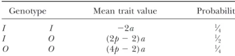
2 I I ⫺2a 1⁄4
O O (4p⫺2)a 1⁄
4 I O⫹ 0 p/2
I O⫺ ⫺2a (1⫺p)/2
O⫺ O⫺ ⫺2a (1⫺p)2/4
O⫺ O⫹ 0 p(1⫺p)/2
quently typed over regions detected in the scan permits O⫹ O⫹ ⫹2a p2/4
the dissection of the variance within theO-derived chro-mosomes and consequently the fine mapping of the QTL. Clearly, the fine-mapping resolution depends on the
ex-and O is V(p)IO ⫽ 2p2. The power to detect the QTL tent to which the QTL segregates within the HS founders.
increases with the variance and hence with the propor-The inbred-outbred design can also be used to map
tion ofO chromosomes that differ fromIat the QTL. modifiers of mutations, which can be introduced intoO
Consequently the optimal detection occurs at p ⫽ 1, by crossing the outbreds to either homozygous or
heter-when all the HS chromosomes carry the increaser QTL ozygous mutant animals. In the former case the design
allele. Whenp ⫽ 0,O is indistinguishable from I and is identical to that described above. In the latter, where
there is no power to detect. theIline carries a mutation that has been maintained
Fine mapping: In the fine-mapping phase, markers
as a heterozygote by backcrossing onto wild-typeI
ani-are typed densely so the QTL is likely to be linked to a mals, then approximately one-half the F1’s have the
mu-marker even on O-descended chromosomes. Thus, in tation. The F2generation is then formed by first
screen-addition to the rather coarse-grained information pro-ing the F1’s for the mutation and either mating each
vided by theI vs. Ocontrast, it is now possible to dissect mutant F1 with a nonmutant, when one-half of the F2
the differences between the HS founders. We denote would carry the mutation and the rest would be normals,
an outbred chromosome carrying an increaser allele as or alternatively intercrossing the F1mutants, to produce
O⫹and a decreaser asO⫺. The possible QTL genotypes, a mix of 25% wild type, 50% mutant heterozygotes, and
trait values, and probabilities are given in Table 2. 25% mutant homozygotes. The choice will depend on
This fully captures all the information about the QTL the nature of the mutation, in particular on the viability
and corresponds to the situation of typing a dense set of mutant homozygotes.
of completely informative markers. The total genetic variance from the above trait distribution is therefore
ANALYSIS
V(p)TOTAL⫽ 2p(2⫺p)a2
To detect a QTL that segregates in the inbred-outbred
cross we calculate the probability that a chromosomal and the extra genetic variance,VOO, explained by fine segment is descended either fromIor from a founder mapping over that explained by detection alone is there-ofO, conditional on the observed genotypes. The proba- fore
bility is calculated using an extension of a multipoint
V(p)OO⫽V(p)TOTAL⫺V(p)IO⫽2p(2⫺p)a2⫺2p2a2⫽4p(1⫺p)a2. dynamic-programming algorithm that we previously
de-veloped to calculateOfounder probabilities for fine
map-Note that the trait variance within the original outbred ping (Mottet al.2000). To simplify the analysis, we first
HS population is describe the ideal situation in which the markers are
completely informative, that is,I and each O founder V(p)HS⫽8p(1⫺ p)a2⫽2V(p) OO, strain carry distinct alleles. We then show how to compute
consistent with the observation that as the F2is 50%O,
descent probabilities when the markers are not fully
in-the variance attributable to O in the inbred-outbred formative, by using information from flanking markers.
cross should be one-half that in a pureO.These
func-QTL detection:For simplicity we assume the presence
tions are graphed in Figure 2a. The genetic variance of an additive diallelic QTL. Alleles descended fromI
available for QTL detection always increases withp, but have effect⫺a, and those descended fromOhave effect
the extra variance explained by the full model attains ⫹a with probability p and ⫺a with probability 1 ⫺ p.
a maximum atp⫽1⁄
2. Whenpis close to 0, thenIand
ThusOchromosomes containing the QTL are a mixture
Oare indistinguishable and there is little power to detect of increasers and decreasers with apparent effect
or localize a QTL; whenpis close to 1, thenOresembles ⫺a(1⫺p)⫹ap⫽a(2p⫺1). Table 1 gives the
distribu-an inbred line—the power to detect is high but the tion of possible F2genotypes, trait values, and
detec-Figure2.—Partitioning of genetic vari-ance in the inbred-outbred cross. The ge-netic variancesVOO(p),VIO(p),VTOTAL(p) are graphed as functions of the proportion pofOchromosomes carrying (a) an ad-ditive increaser QTL with effect⫹1. All I chromosomes carry decreaser alleles with effect⫺1. (b) A dominant increaser QTL with effect⫹1. AllIchromosomes carry recessive alleles with effect 0.
tion. Consequently this experimental design is most ap- V(p)HS⫽p(1⫺ p)2(2⫺p)a2
propriate when about one-half the founders ofOcarry
V(p)TOTAL⫽ p(2⫺ p)2(4⫺p)a2/16
QTL alleles that differ fromI.
The sample size required for QTL detection will be V(p)IO⫽p2(8⫺8p⫹ 3p2)a2/16
equivalent to that required in an F2 cross between two V(p)
OO ⫽(1⫺ p)(4⫺3p⫹p2)a2/4 inbred strains with genetic variance equal to V(p)IO,
rather than V(p)TOTALorV(p)HS. The variance available (Figure 2b), and consequently any intermediate
be-tween dominance and additivity should also follow the for QTL detection in the F2can be significantly less than
the genetic variance originally present in the HS. For same pattern.
Multipoint mapping:The analysis of real data is
com-example, if p⫽ 1⁄
2 and V(1⁄2)OO ⫽ 5%, thenV(1⁄2)TOTAL⫽
6.67%, butV(1⁄
2)IO⫽1.67%. plicated by the issue of marker informativity. Not all
strains withinOor between theOandIare distinguish-Qualitatively similar behavior holds if the QTL is
sequently the variances derived above are idealizations the trait of Iand each founderOfis estimated by least squares. Differences between the estimates are evalu-that only give upper bounds on the power of the
inbred-outbred cross. ated with anF-test. Although the bulk of the
fine-map-ping information is due to differences between the Previously we have shown how to use a multipoint
dy-namic-programming algorithm, implemented in the pro- founders ofO, there is also some information from the
I/O contrast. Hence we estimate the QTL position by gram HAPPY, to determine the probability of each
found-ing haplotype at any locus (Mott et al. 2000). The the marker interval with the smallest ANOVAP value from fitting a full model with bothIandO present. analysis requires the phenotypes and marker genotypes
of the final generation and the marker alleles ofIand The overall efficiency Pr(r) of the method is defined as the probability that a QTL will be both detected with the founder strains used to make the HS. Pedigree
infor-mation is not required. Use of flanking marker data in a genome-widePvalue⬍1.5% (i.e., at least one marker interval has an ANOVAPvalue⬍10⫺4) and fine mapped
this way alleviates the problem of marker informativity
and significantly increases the power to detect and fine to within r 1-cM intervals of its true position. In this study localization to within 3 cM is deemed to be a map QTL.
We now describe the necessary modifications re- success.
quired to analyze an inbred-outbred cross. The QTL-detection step of the analysis is an F2 cross between I
SIMULATIONS
andO, in whichOis treated as if it were a single strain
(albeit no longer inbred), so the cross is like a heteroge- We investigated the power of the inbred-outbred cross by computer simulation. First,Opopulations were gen-neous stock formed from two foundersIandOand just
two generations old. It can then be analyzed using the erated by intercrossing eight inbred founders for 60 generations, keeping 40 mating pairs in each generation original version of HAPPY.
For the fine-mapping step it is necessary to model the and avoiding brother-sister matings. Each individual was simulated as a 100-cM diploid chromosome. Individuals different scales of recombination present within and
from the finalO generation were then crossed with a between chromosomal segments descended from Ior
pure inbred line, either identical to one of the eightO O.In Mottet al.(2000) the genotypes were modeled
founders or completely distinct, in the sense that each as a realization of a hidden Markov chain, in which the
marker distinguished betweenIandO.Real crosses will ancestral haplotypes were the hidden states and the
lie between these extremes. marker genotypes the observed data. We use a similar
The 80O animals were mated withIto produce 400 formulation for the inbred-outbred cross, except that
F1offspring, which were crossed to produce F2
popula-the priors and transition probabilities between founder
tions of 1000, 1500, and 2000 subjects. Microsatellite states are no longer uniform, but instead depend on
markers spaced 1 cM apart were typed across the chro-whether the states areIorO.The prior probability that
mosome. The distribution of alleles per marker was a locus is descended fromIorO is1⁄
2. The probability
modeled on the real microsatellites used inTalbotet
of descent from any particularOfounder, sayOf, isS/2,
al.(1999) and ranged from 2 to 5 with a mean of 3.80. where S is the number of founders. We assume the
An additive QTL accounting for 5, 7.5, or 10% of the Haldane model of recombination applies: in an interval
total phenotypic variance in the F2 was placed midway
of lengthdmorgans, the probability that no
recombina-between a randomly chosen pair of adjacent markers. tion events occur in a single meiosis is e⫺d. In an O
One-half of theOfounders, chosen at random, carried interval intercrossed overGgenerations the probability
increaser alleles and the remainder carried decreasers. of no recombination is e⫺Gd. Consequently, the prior
Genetic drift during the breeding protocol meant that probabilityrm(s|) that the ancestral state on a
chromo-the proportionpof chromosomes carrying the increaser some at some markerm⫹1 iss, given it isat marker
in the finalO generation varied considerably between
m, distance dapart, and before any genotype
informa-simulations. Inⵑ5% of simulations the QTL drifted to tion atm⫹ 1 is considered, is
fixation, and these runs were discarded. Environmental
rm(I|I)⫽ e⫺d⫹(1⫺ e⫺d)/2 variance was normally distributed and uncorrelated with
the QTL. A total of 1000 simulations were performed
rm(Of|I)⫽ (1⫺e⫺d)/2S
for each combination of parameters.
rm(I|Of)⫽ (1⫺e⫺d)/2 QTL detection:QTL detection was performed using
a subset of 10 markers spaced 10 cM apart across the
rm(Og|Of)⫽ (1⫺e⫺d)/2S⫹e⫺d(␦gfe⫺Gd⫹1⫺e⫺Gd)/S,
chromosome, corresponding to a genome scan of 150 where␦gfis the delta function. Apart from these changes, markers (taking the mouse genome as 1500 cM). QTL
the statistical development is similar to Mott et al. detection was deemed successful if the HAPPY analysis
(2000). of the 10 markers identified an interval with an ANOVA
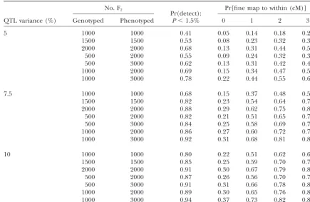
TABLE 3
Power to detect and fine map QTL:I,Onot distinct
No. F2 Pr[fine map to within (cM)]
Pr(detect):
QTL variance (%) Genotyped Phenotyped P⬍1.5% 0 1 2 3
5 1000 1000 0.41 0.05 0.14 0.18 0.23
1500 1500 0.53 0.08 0.23 0.32 0.38
2000 2000 0.68 0.13 0.31 0.44 0.52
500 2000 0.55 0.09 0.24 0.32 0.37
500 3000 0.62 0.13 0.31 0.42 0.48
1000 2000 0.69 0.15 0.34 0.47 0.53
1000 3000 0.78 0.22 0.44 0.55 0.63
7.5 1000 1000 0.68 0.15 0.37 0.48 0.54
1500 1500 0.82 0.23 0.54 0.64 0.71
2000 2000 0.88 0.29 0.62 0.75 0.81
500 2000 0.82 0.21 0.51 0.65 0.71
500 3000 0.84 0.25 0.58 0.69 0.74
1000 2000 0.86 0.27 0.60 0.72 0.77
1000 3000 0.92 0.31 0.68 0.81 0.86
10 1000 1000 0.80 0.22 0.51 0.62 0.69
1500 1500 0.85 0.25 0.59 0.70 0.76
2000 2000 0.91 0.30 0.67 0.79 0.85
500 2000 0.87 0.26 0.56 0.70 0.76
500 3000 0.91 0.31 0.66 0.78 0.85
1000 2000 0.89 0.30 0.65 0.76 0.83
1000 3000 0.94 0.37 0.73 0.82 0.88
Shown is the probability to detect and fine map a QTL at a 1.5% genome-wide significance level, over a range of QTL effects and numbers of F2animals genotyped/phenotyped, and when the inbred lineIhas marker alleles indistinguishable from one of the founders ofO.Each probability is estimated from 1000 simulations of the inbred-outbred cross.
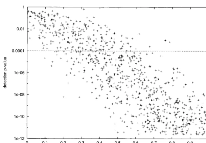
than is normal (5%) because we wished to reduce the the probability of detecting the QTL increases with p
as expected, but that there is considerable variation in risk of false positives. In addition, the threshold is
con-servative because the tests are not independent. the significance level achieved at a givenp, due perhaps to variation in the information content of markers near The power to detect the QTL is given in Tables 3 (I
is identical to one of the founders ofO) and 4 (Iand the QTL. The effect of genetic drift on the QTL is also shown; starting fromp⫽1⁄
2in the founders,pis roughly Oare completely distinguishable). Power increases with
sample size and genetic variance and when I is separ- uniformly distributed in the final generation of the HS.
Fine mapping:QTL fine mapping using 100 markers
able from O. For example, for a QTL accounting for
5% of the phenotypic variance, genotypes from 2000 spaced 1 cM apart across the chromosome was
per-formed only when the QTL detection was significant. animals produce 80% power to detect the QTL with
markers that can distinguish I fromO compared with The position of the QTL was estimated as the fine-map interval with the smallest ANOVAPvalue, using a only 68% otherwise.
Tables 3 and 4 also show that power is increased sig- version of HAPPY modified to analyze the nonhomoge-neous chromosome structure. The fine-map error was nificantly by selective genotyping, i.e., phenotyping a
larger number of F2’s and then genotyping only the defined as the number of marker intervals separating
the QTL’s true and predicted positions. A fine-map extremes. Simulations were performed with populations
of 1000, 2000, and 3000 F2individuals, from which only error of n intervals implies that the distance between
the true and predicted positions lies between n ⫺ 1⁄ 2
the extremes (500/3000 ⫽ 17%, 500/2000 ⫽ 25%,
1000/2000⫽50%, and 1000/3000⫽33%) were geno- andn⫹1⁄
2 cM.
The resolution of the fine-mapping step over a range typed. A 5% QTL can be detected with 77% power in
a selected sample of 1000 out of 2000 individuals. of QTL effects, sample sizes, and selection regimes is summarized in Tables 3 and 4. The resolution is ex-In Figure 3 the detectionPvalue is plotted againstp,
the proportion of chromosomes in the final HS genera- pressed in terms of the probability that the QTL is both detected and fine mapped to a 1-cM interval 0, 1, 2, or tion that carry the modifier, for 5% QTL effect, 1500
TABLE 4
Power to detect and fine map QTL:I,Odistinct
No. F2 Pr[fine map to within (cM)]
Pr(detect):
QTL variance (%) Genotyped Phenotyped P⬍1.5% 0 1 2 3
5 1000 1000 0.59 0.10 0.25 0.34 0.40
1500 1500 0.69 0.15 0.38 0.47 0.52
2000 2000 0.80 0.22 0.51 0.63 0.69
500 2000 0.70 0.15 0.39 0.49 0.55
500 3000 0.77 0.19 0.42 0.56 0.63
1000 2000 0.77 0.20 0.46 0.58 0.65
1000 3000 0.86 0.25 0.55 0.68 0.76
7.5 1000 1000 0.60 0.12 0.30 0.40 0.44
1500 1500 0.71 0.18 0.40 0.50 0.56
2000 2000 0.81 0.20 0.48 0.62 0.69
500 2000 0.71 0.16 0.40 0.50 0.57
500 3000 0.79 0.20 0.46 0.58 0.66
1000 2000 0.78 0.21 0.42 0.57 0.65
1000 3000 0.86 0.21 0.54 0.67 0.75
10 1000 1000 0.69 0.16 0.39 0.49 0.54
1500 1500 0.79 0.20 0.47 0.61 0.67
2000 2000 0.85 0.27 0.55 0.70 0.76
500 2000 0.77 0.17 0.45 0.58 0.65
500 3000 0.85 0.22 0.49 0.64 0.72
1000 2000 0.83 0.22 0.52 0.65 0.73
1000 3000 0.90 0.27 0.58 0.73 0.80
Shown is the probability to detect and fine map a QTL at a 1.5% genome-wide significance level, over a range of QTL effects and numbers of F2animals genotyped/phenotyped, and when the inbred lineIhas marker alleles distinguishable from all of the founders ofO.Each probability is estimated from 1000 simulations of the inbred-outbred cross.
efficiency increases with QTL effect and sample size, Oseparable there is a 69% probability of fine mapping the QTL to within 3 cM and a 65% probability if only marker informativity, and when extremes are genotyped.
Thus for a 5% effect QTL with 2000 animals andIand the extreme 1000/2000 are genotyped. Table 4 shows
Figure4.—Spatial distribution of QTL fine-map precision. Data are from 1000 simulations of the inbred-outbred cross for an additive 5% QTL effect size, 1500 F2animals, and markers that can distin-guishIfromO, expressed as the proba-bility that the QTL was fine mapped, given it was detected.
that there is only a small reduction in power with selec- would be able to fine map over one-half of these. Conse-quently the method should yield a sufficient number tive genotyping, yet at a significant reduction in
genotyp-ing cost. Figure 4 shows the distribution of the fine- of fine-mapped candidate regions for further study in an average-sized laboratory.
mapping error for one simulation set.
In a few instances the fine-mapping step completely The analysis relies on knowing the probability of whether the inbred line or one of the founders of the HS failed to localize the QTL. In these cases usually the
fine-mapping P value was almost flat over a wide block of was present at any position on the genome, conditional upon the observed marker data. We implemented the intervals, indicating behavior akin to a detection
experi-ment. Consequently it should be possible to identify calculation as a dynamic-programming algorithm in the HAPPY package, which is able to carry out a complete likely failures from the shape of the fine-map curve or
by bootstrapping. analysis of an inbred-outbred cross, including an analysis
of variance to test for QTL significance in each marker interval. The required input data are the phenotypes
DISCUSSION and marker genotypes from the F
2 animals, the
geno-types of the inbred progenitor strains of the HS and of We have presented an experimental design to detect
the inbred line, and the genetic distances between the and fine map QTL segregating in HS outbred mice.
markers. No pedigree data are used. The package is The method overcomes a potential limitation of using
available free from http://www.well.ox.ac.uk/happy. the HS for fine mapping, namely the prohibitively large
The major advantage of the inbred-outbred cross over number of genotypes required for a genome scan, and
other experimental designs is that it provides high QTL in addition enables the simultaneous detection and fine
genome-wide mapping resolution in a short period of mapping of modifier loci when the inbred line used in
time. One obvious application will be in mapping mod-the cross carries a mutation. Depending on mod-the effect
ifiers that influence the phenotype either of transgenic size of the QTL, in the order of 1000–2000 animals are
models of human disease or of mutants produced by required to detect a QTL with 80% power. Selective
mouse mutagenesis projects. A disadvantage is that un-genotyping reduces this number to nearer 1000. In most
less the QTL segregates within the HS, the ability of the cases there is at least a 50% probability that the QTL
inbred-outbred cross to fine map the locus will be no will be both detected and fine mapped to within 3 cM.
better than a standard F2 or backcross.
In general we expect to find multiple loci influencing
This strategy is within the reach of most laboratories. a trait. For instance, in our previous work (Mottet al.
The expense of performing the inbred-outbred cross, 2000) we fine mapped five loci that had been identified
in the form described here, is divided between animal previously in F2 intercrosses. More QTL should
segre-and genotyping costs. The strategy requires 400 F1’s as
gate in the HS than in an intercross between only two
200 breeding pairs and phenotypes from ⵑ1500 F2’s.
inbred lines, so we expect a genome scan using the
The genome scan, without selection, using 150 markers, eight founders of the HS to detect perhaps double this
a furtherⵑ50 markers are needed for each QTL identi- Third, we stress the advantages of using markers whose alleles are different in the inbred line and the outbreds. fied or 75,000 genotypes for the 1500 mice. If there are
10 QTL in the genome and 80% are detected, then In practice, most mouse knockout mutants originate on a 129 strain, which is not a founder in any current HS ⵑ750,000 genotypes will be required in total. Selection
significantly reduces the amount of genotyping required population. Consequently it should be possible to choose, at least in the detection phase, informative markers for (by up to 50%), at the cost of approximately doubling
the phenotyping effort and F2 animal costs. Alterna- mapping crosses between knockout lines and the HS.
Microsatellite markers are preferable to SNPs because tively, genotyping could be reduced by one-quarter
with-out selection, once the QTL has been localized to of their cost and information content. Because a SNP has only two alleles, compared with about four in a ⵑ10–20 cM, by noting thatⵑ25% of the animals should
be inbred line homozygotes I-I over the region and microsatellite in the HS, we would need to double the number of markers in the fine-mapping phase, but the hence cannot contribute to the fine mapping. These
individuals are identifiable from the genome scan and ease and accuracy of SNP typing may make them the marker of choice in the future.
need not be genotyped further. Hence the effort could
be easily reduced to about half a million genotypes. We have not explored all possible extensions of this strategy and there are likely to be experimental and Our simulations point to some important
considera-tions for the experimental design. First, obtaining ade- analytical modifications that will improve the efficiency of both detection and high resolution mapping. These quate power to detect a QTL in the inbred-outbred
cross requires more animals than for an F2intercross. include variations in the breeding design and the use
of variance components approaches (Searleet al.1992) However, it should be noted that the QTL effect sizes
are not directly comparable between the two designs. to extract information from families (McPeek 2000). Furthermore, genotyping the F1generation may enable
All the QTL variance in the F2 intercross is available
for QTL detection, whereas only a part contributes to us to detect genotype errors and determine the phase of the F2genotypes, which should increase power. Mixture
detection in the inbred-outbred cross, depending on
the proportionpof HS chromosomes carrying a differ- models, fitted using Markov chain Monte Carlo algo-rithms, may also be useful, for instance, when a number ent allele from the inbred. We cannot know or control
that proportion. The variance available for QTL detec- of linked QTL are present (Lange1997;Sillanpaaand
Arjas1998;XuandYi2000;Baldinget al.2001). tion in the F2can be significantly less than the genetic
variance originally present in the HS. For example, if An alternative breeding strategy would be to use F1
animals for fine mapping, instead of the F2generation p⫽1⁄
2and the QTL accounts for 5% of the total variance
in the F2 generation, then the variance available for (as discussed briefly inMottet al.2000). However, for
an additive QTL the genetic variance in the F1will be
detection is⬍2%. It should be recognized that there is
some ambiguity in the definition of genetic variance: less than in the F2, so more animals will be required to
obtain the same accuracy as the F2strategy. Furthermore
different results might be obtained if, for instance, the
genetic variance were fixed in the initial HS generation the detection step still requires genotypes from the F2
generation. On the other hand, typing F1’s may be more
rather than in the F2. We deliberately ignored simulation
runs that had drifted to fixation at the QTL; were they appropriate when mapping modifiers with dominant or epistatic effects (Abneyet al.2000). Another possibility taken into account, the power might be reduced slightly.
Second, fine-mapping resolution can be increased would be to use an advanced intercross line, such as an F3or F4in place of the F2; more of the genetic variance
further by spacing markers closer together, although
there is a limit to the density of markers that can be would be then available for fine mapping, but at the cost of additional breeding and a higher density of markers usefully employed. Theoretically, resolution depends
on the structure of the haplotypes present in a region required during the genome scan.
In this study we used variants of one experimental surrounding the QTL in the HS population, itself a
function of the number of generationsGsince the HS design, namely 40 HS mating pairs and 400 F1animals.
This is appropriate for a modifier screen in which a was founded and the effective HS population size. This
must be⬍100/GNcM, whereN is the number of HS litter of 10 F1’s is bred from each HS animal, of which
one-half carry the mutation. However, if the mutant chromosomes. Using 40 mating pairs over 60
genera-tions gives a lower bound of 100/2400 or 0.02 cM. Ge- reduces fertility it may be necessary to breed the F2’s
from a smaller number of F1’s or to produce more litters
netic drift, operating to decrease heterozygosity over
time, makes this limit highly improbable. Our experi- of F1’s. These may alter the power to detect and fine map
QTL. Simulations (not shown) indicate it is important to ence of mapping QTL in the HS suggests that markers
spaced closer than 0.1 cM do not help to increase resolu- maintain the genetic heterogeneity in the F1generation.
Since there are 160 HS chromosomes present, 320 F1’s
tion. Furthermore the current mouse genetic and
radia-tion-hybrid maps cannot resolve the order of very closely are required to give at least the possibility that all this genetic material is still present in the F1 generation.
spaced markers, although this will change when the
approach-Darvasi, A., andM. Soller,1995 Advanced intercross lines, an
ing 1 cM throughout the genome represents a
substan-experimental population for fine genetic mapping. Genetics141:
tial advance over competing methodologies. However, 1199–1207.
Flint, J.,andR. Mott,2001 Finding the molecular basis of
quantita-investigations in Drosophila suggest that, rather than
tive traits: successes and pitfalls. Nat. Rev. Genet.2:437–445.
being caused by a single molecular change, a QTL can
Lange, K.,1997 Mathematical and Statistical Methods for Genetic
Analy-comprise a tight cluster of interacting polymorphisms sis.Springer Verlag, New York.
Long, A. D., S. L. Mullaney, T. F. MackayandC. H. Langley, (Longet al.1996) and it is likely that mammalian QTL
1996 Genetic interactions between naturally occurring alleles
will exhibit a similar hidden complexity. Therefore, in
at quantitative trait loci and mutant alleles at candidate loci
af-addition to fine-scale genetic mapping, QTL analysis fecting bristle number inDrosophila melanogaster. Genetics144:
1497–1510.
calls for an integrated repertoire of tools, including the
McClearn, G. E.,andW. Meredith,1970 The use of isogenic and
completed and fully annotated sequences of the human
heterogenic mouse stocks in behavioral research, pp. 3–22 in
and mouse genomes, gene expression data (Aitmanet Contributions to Behavior-Genetic Analysis: The Mouse as Prototype, edited byG. T. Lindzey.Appleton Century Crofts, New York. al. 1999), and chromosomal engineering techniques
McPeek, M. S.,2000 From mouse to human: fine mapping of
quanti-(Ramirez-Soliset al.1995). Determining the molecular
tative trait loci in a model organism. Proc. Natl. Acad. Sci. USA
basis of the QTL remains a formidable challenge and 97:12389–12390.
Mott, R., C. J. Talbot, M. G. Turri, A. C. CollinsandJ. Flint, will occupy researchers for some time to come.
2000 From the cover: a method for fine mapping quantitative This work was supported by a grant from the Wellcome Trust. trait loci in outbred animal stocks. Proc. Natl. Acad. Sci. USA97:
12649–12654.
Ramirez-Solis, R., P. LiuandA. Bradley, 1995 Chromosome engi-neering in mice. Nature378:720–724.
LITERATURE CITED Searle, S. R. C., G. CasellaandC. E. McCulloch,1992 Variance Components.Wiley-Interscience, New York.
Abney, M., M. S. McPeekandC. Ober,2000 Estimation of variance Sillanpaa, M. J.,andE. Arjas,1998 Bayesian mapping of multiple components of quantitative traits in inbred populations. Am. J. quantitative trait loci from incomplete inbred line cross data. Hum. Genet.66:629–650. Genetics148:1373–1388.
Aitman, T. J., A. M. Glazier, C. A. Wallace, L. D. Cooper, P. J. Talbot, C. J., A. Nicod, S. S. Cherny, D. W. Fulker, A. C. Collins Norsworthyet al., 1999 Identification of Cd36 (Fat) as an et al., 1999 High-resolution mapping of quantitative trait loci insulin-resistance gene causing defective fatty acid and glucose in outbred mice. Nat. Genet.21:305–308.
metabolism in hypertensive rats. Nat. Genet.21:76–83. Threadgill, D. W., A. A. Dlugosz, L. A. Hansen, T. Tennenbaum, U.
Alpert, K. B.,andS. D. Tanksley,1996 High-resolution mapping Lichtiet al., 1995 Targeted disruption of mouse EGF receptor: and isolation of a yeast artificial chromosome contig containing effect of genetic background on mutant phenotype. Science269: fw2.2: a major fruit weight quantitative trait locus in tomato. Proc. 230–234.
Natl. Acad. Sci. USA93:15503–15507. Wells, C.,andS. D. Brown,2000 Genomics meets genetics: towards
Balding, D. J., C. CanningsandM. Bishop(Editors), 2001 Hand- a mutant map of the mouse. Mamm. Genome11:472–477. book of Statistical Genetics.John Wiley & Sons, Chichester, UK. Xu, S.,andN. Yi,2000 Mixed model analysis of quantitative trait
Darvasi, A.,1997 Interval-specific congenic strains (ISCS): an ex- loci. Proc. Natl. Acad. Sci. USA97:14542–14547. perimental design for mapping a QTL into a 1-centimorgan