Parameter Selection Methods in Inverse Problem Formulation
H. T. Banks1 and Ariel Cintr´on-Arias1,21Center for Research in Scientific Computation Center for Quantitative Sciences in Biomedicine
Department of Mathematics North Carolina State University
Raleigh, NC 27695-8212 and
2Department of Mathematics and Statistics East Tennessee State University
Johnson City, TN 37614-0663 June 19, 2010
Abstract
We discuss methods for a priori selection of parameters to be estimated in inverse problem formulations (such as Maximum Likelihood, Ordinary and Generalized Least Squares) for dynamical systems with numerous state variables and an even larger num-ber of parameters. We illustrate the ideas with an in-host model for HIV dynamics which has been successfully validated with clinical data and used for prediction.
1 Introduction
There are many topics of great importance and interest in the areas of modeling and inverse problems which are properly viewed as essential in the use of mathematics and statistics in scientific inquiries. A brief, noninclusive list of topics include the use of traditional sensitivity functions (TSF) and generalized sensitivity functions (GSF) in experimental design (what type and how much data is needed, where/when to take observations) [9, 10, 11, 16, 56], choice of mathematical models and their parameterizations (verification, validation, model selection and model comparison techniques) [7, 12, 13, 17, 21, 22, 24, 25, 41], choice of statistical models (observation process and sampling errors, residual plots for statistical model verification, use of asymptotic theory and bootstrapping for computation of standard errors, confidence intervals) [7, 14, 30, 31, 54, 55], choice of cost functionals (MLE, OLS, WLS, GLS, etc.,) [7, 30], as well as parameter identifiability and selectivity. There is extensive literature on each of these topics and many have been treated in surveys in one form or another ([30] is an excellent monograph with many references on the statistically related topics) or in earlier lecture notes [7].
We discuss here an enduring major problem: selection of which model parameters can be readily and reliably (with quantifiable uncertainty bounds) estimated in an inverse prob-lem formulation. This is especially important in many areas of biological modeling where often one has large dynamical systems (many state variables), an even larger number of unknown parameters to be estimated and a paucity of longitudinal time observations or data points. As biological and physiological models (at the cellular, biochemical pathway or whole organism level) become more sophisticated (motivated by increasingly detailed understanding - or lack thereof - of mechanisms), it is becoming quite common to have large systems (10-20 or more differential equations), with a plethora of parameters (25-100) but only a limited number (50-100 or fewer) of data points per individual organism. For example, we find models for the cardiovascular system [16, Chapter 1] (where the model has 16 state variables and 22 parameters) and [50, Chapter 6] (where the model has 22 states and 55 parameters), immunology [48] (8 states, 24 parameters), metabolic pathways [32] (8 states, 35 parameters) and HIV progression [8, 43] (8 & 6 states, 11 & 8 parameters, respectively). Fortunately, there is a growing recent effort among scientists to develop quantitative methods based on sensitivity, information matrices and other sta-tistical constructs (see for example [9, 10, 11, 23, 28, 37, 38, 59]) to aid in identification or parameter estimation formulations. We discuss here one approach using sensitivity ma-trices and asymptotic standard errors as a basis for our developments. To illustrate our discussions, we will use a recently developed in-host model for HIV dynamics which has been successfully validated with clinical data and used for prediction [4, 8].
33, 39, 44, 46, 52, 53]. These early investigations and results were focused primarily on engineering applications, although much interest in other areas (e.g., oceanography, biol-ogy) has prompted more recent inquiries for both linear and nonlinear dynamical systems [5, 15, 29, 35, 42, 47, 58, 59, 60, 61].
1.1 A Mathematical Model for HIV Progression with Treatment Inter-ruption
We summarize and use as an illustrative example one of the many dynamic models for HIV progression found in an extensive literature (e.g., see [1, 2, 3, 4, 8, 20, 26, 49, 51, 57] and the many references therein). For our example model, the dynamics of in-host HIV are described by the interactions between uninfected and infected type 1 target cells (𝑇1 and 𝑇∗
1) (CD4+ T-cells), uninfected and infected type 2 target cells (𝑇2 and 𝑇2∗) (such as macrophages or memory cells, etc.), infectious free virus 𝑉𝐼, and immune response 𝐸
(cytotoxic T-lymphocytes CD8+) to the infection. This model, which was developed and studied in [1, 4] and later extended in subsequent efforts (e.g., see [8]), is essentially one suggested in [26], but includes an immune response compartment and dynamics as in [20]. The model equations are given by
˙
𝑇1=𝜆1−𝑑1𝑇1−(1−¯𝜖1(𝑡))𝑘1𝑉𝐼𝑇1 ˙
𝑇2=𝜆2−𝑑2𝑇2−(1−𝑓¯𝜖1(𝑡))𝑘2𝑉𝐼𝑇2 ˙
𝑇∗
1 = (1−¯𝜖1(𝑡))𝑘1𝑉𝐼𝑇1−𝛿𝑇1∗−𝑚1𝐸𝑇1∗ ˙
𝑇∗
2 = (1−𝑓¯𝜖1(𝑡))𝑘2𝑉𝐼𝑇2−𝛿𝑇2∗−𝑚2𝐸𝑇2∗ ˙
𝑉𝐼 = (1−¯𝜖2(𝑡))103𝑁𝑇𝛿(𝑇1∗+𝑇2∗)−𝑐𝑉𝐼
−(1−¯𝜖1(𝑡))103𝑘1𝑇1𝑉𝐼 −(1−𝑓¯𝜖1(𝑡))103𝑘2𝑇2𝑉𝐼
˙
𝐸 =𝜆𝐸 +(𝑇𝑏𝐸∗(𝑇1∗+𝑇2∗)
1+𝑇2∗)+𝐾𝑏𝐸−
𝑑𝐸(𝑇1∗+𝑇2∗)
(𝑇∗
1+𝑇2∗)+𝐾𝑑𝐸−𝛿𝐸𝐸,
(1)
together with an initial condition vector (𝑇1(0), 𝑇1∗(0), 𝑇2(0), 𝑇2∗(0), 𝑉𝐼(0), 𝐸(0))𝑇 .
The differences in infection rates and treatment efficacy help create a low, but non-zero, infected cell steady state for 𝑇∗
2, which is compatible with the idea that macrophages or memory cells may be an important source of virus after T-cell depletion. The popula-tions of uninfected target cells 𝑇1 and 𝑇2 may have different source rates 𝜆𝑖 and natural
period of time, implemented by considering separate treatment functions𝑢1(𝑡), 𝑢2(𝑡) in the treatment factors.
As in [1, 4], for our numerical investigations we consider a log-transformed and reduced version of the model. This transformation is frequently used in the HIV modeling literature because of the large differences in orders of magnitude in state values in the model and the data and to guarantee non-negative state values as well as because of certain probabilistic considerations (for further discussions see [4]). This results in the nonlinear system of differential equations
𝑑𝑥1 𝑑𝑡 =
10−𝑥1
ln(10)(𝜆1−𝑑110𝑥1 −(1−𝜀¯1(𝑡))𝑘110𝑥510𝑥1) (2) 𝑑𝑥2
𝑑𝑡 =
10−𝑥2
ln(10)((1−𝜀¯1(𝑡))𝑘110𝑥510𝑥1−𝛿10𝑥2 −𝑚110𝑥610𝑥2) (3) 𝑑𝑥3
𝑑𝑡 =
10−𝑥3
ln(10)(𝜆2−𝑑210𝑥3 −(1−𝑓𝜀¯1(𝑡))𝑘210𝑥510𝑥3) (4) 𝑑𝑥4
𝑑𝑡 =
10−𝑥4
ln(10)((1−𝑓𝜀¯1(𝑡))𝑘210𝑥510𝑥3 −𝛿10𝑥4−𝑚210𝑥610𝑥4) (5) 𝑑𝑥5
𝑑𝑡 =
10−𝑥5
ln(10)((1−𝜀¯2(𝑡))103𝑁𝑇𝛿(10𝑥2 + 10𝑥4)−𝑐10𝑥5 −
(1−𝜀¯1(𝑡))𝜌1103𝑘110𝑥110𝑥5−(1−𝑓𝜀¯1(𝑡))𝜌2103𝑘210𝑥310𝑥5) (6) 𝑑𝑥6
𝑑𝑡 =
10−𝑥6
ln(10)
(
𝜆𝐸+ 𝑏𝐸(10
𝑥2 + 10𝑥4)
(10𝑥2 + 10𝑥4) +𝐾𝑏10
𝑥6− 𝑑𝐸(10𝑥2 + 10𝑥4)
(10𝑥2 + 10𝑥4) +𝐾𝑑10
𝑥6 −𝛿
𝐸10𝑥6 )
, (7)
where the changes of variables are defined by
𝑇1= 10𝑥1, 𝑇1∗ = 10𝑥2, 𝑇2 = 10𝑥3, 𝑇2∗ = 10𝑥4, 𝑉𝐼 = 10𝑥5, 𝐸 = 10𝑥6. (8)
We note that this model contains six state variables and twenty-two (in general, unknown) system parameters given by
𝜃2= (𝜆1, 𝑑1, 𝜖1, 𝑘1, 𝜆2, 𝑑2, 𝑓, 𝑘2, 𝛿, 𝑚1, 𝑚2, 𝜖2, 𝑁𝑇, 𝑐, 𝜌1, 𝜌2, 𝜆𝐸, 𝑏𝐸, 𝐾𝑏, 𝑑𝐸, 𝐾𝑑, 𝛿𝐸).
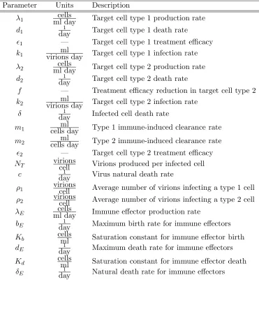
A list of the model parameters along with units of these model parameters are given below in Table 1.
The initial conditions for equations (2)–(7) are denoted by𝑥𝑖(𝑡0) =𝑥0𝑖, for𝑖= 1, . . . ,6.
We will also consider the initial conditions as unknowns and we use the following notation for the vector of parameters and initial conditions:
𝜃= (𝜃1, 𝜃2) where
Table 1: Parameters for the HIV model.
Parameter Units Description
𝜆1 ml daycells Target cell type 1 production rate 𝑑1 day1 Target cell type 1 death rate
𝜖1 — Target cell type 1 treatment efficacy 𝑘1 virions day Target cell type 1 infection rateml 𝜆2 ml daycells Target cell type 2 production rate 𝑑2 day1 Target cell type 2 death rate
𝑓 — Treatment efficacy reduction in target cell type 2 𝑘2 virions day Target cell type 2 infection rateml
𝛿 day1 Infected cell death rate
𝑚1 cells dayml Type 1 immune-induced clearance rate 𝑚2 cells dayml Type 2 immune-induced clearance rate
𝜖2 — Target cell type 2 treatment efficacy 𝑁𝑇 virionscell Virions produced per infected cell
𝑐 day1 Virus natural death rate
𝜌1 virionscell Average number of virions infecting a type 1 cell 𝜌2 virionscell Average number of virions infecting a type 2 cell 𝜆𝐸 ml daycells Immune effector production rate
𝑏𝐸 day1 Maximum birth rate for immune effectors
𝐾𝑏 cellsml Saturation constant for immune effector birth
𝑑𝐸 day1 Maximum death rate for immune effectors
𝐾𝑑 cellsml Saturation constant for immune effector death
2 Statistical Models for the Observation Process
One has errors in any data collection process and the presence of this error is reflected in any parameter estimation results one might obtain. To understand and treat this, one usually specifies a statistical model for the observation process in addition to the mathe-matical model representing the dynamics. To illustrate ideas here we use ordinary least squares (OLS) consistent with an error model for absolute error in the observations. For a discussion of other frameworks (maximum likelihood in the case of known error distri-butions, generalized least squares appropriate for relative error models) see [7]. Here the OLS estimation is based on the mathematical model for in-host HIV dynamics described above. The observation process is formulated assuming there exists a vector 𝜃0 ∈ ℝ𝑝, re-ferred to as thetrue parameter vector, for which the model describes the log-scaled total number of CD4+ T-cells (uninfected and infected) exactly. It is also reasonably assumed that each of𝑛longitudinal observations {𝑌𝑖}𝑛
𝑖=1 is affected by random deviations from the true underlying process. That is, if the mathematical model output is denoted by
𝑧(𝑡𝑖;𝜃0) = log10
(
10𝑥1(𝑡𝑖;𝜃0)+ 10𝑥2(𝑡𝑖;𝜃0)), (9)
then the statistical model for the scalar observation process is
𝑌𝑖 =𝑧(𝑡𝑖;𝜃0) +ℰ𝑖 for𝑖= 1, . . . , 𝑛. (10)
The errorsℰ𝑖 are assumed to be random variables satisfying the following assumptions:
(i) the errorsℰ𝑖 have mean zero,𝐸[ℰ𝑖] = 0;
(ii) the errorsℰ𝑖 have finite common variance, var(ℰ𝑖) =𝜎02<∞;
(iii) the errors ℰ𝑖 are independent (i.e., cov(ℰ𝑖,ℰ𝑗) = 0 whenever 𝑖 ∕= 𝑗) and identically distributed.
Assumptions (i)–(iii) imply that the mean of the observation is equal to the model output, 𝐸[𝑌𝑖] =𝑧(𝑡𝑖;𝜃0), and the variance in the observations is constant in time, var(𝑌𝑖) =𝜎02.
The estimator 𝜃𝑂𝐿𝑆 =𝜃𝑛𝑂𝐿𝑆 minimizes 𝑛 ∑
𝑖=1
[𝑌𝑖−𝑧(𝑡𝑖;𝜃)]2. (11)
From [54] we find that under a number of regularity and sampling conditions, as𝑛→ ∞, 𝜃𝑂𝐿𝑆 is approximately distributed according to a multivariate normal distribution, i.e.,
where Σ𝑛
0 =𝜎20[𝑛Ω0]−1∈ℝ𝑝×𝑝 and
Ω0 = lim𝑛→∞𝑛1𝜒𝑛(𝜃0)𝑇𝜒𝑛(𝜃0). (13)
Asymptotic theory requires existence of this limit and non-singularity of Ω0. The 𝑝×𝑝 matrix Σ𝑛
0 is the covariance matrix, and the𝑛×𝑝matrix𝜒𝑛(𝜃0) is known as thesensitivity matrixof the system, and is defined as
𝜒𝑛
𝑖𝑗(𝜃0) = ∂𝑧∂𝜃(𝑡𝑖;𝜃)
𝑗
𝜃=𝜃0
1≤𝑖≤𝑛, 1≤𝑗 ≤𝑝. (14)
If 𝑔 ∈ℝ6 denotes the right-side of Equations (2)–(7), then numerical values of 𝜒𝑛(𝜃) are
readily calculated, for a particular 𝜃, by solving 𝑑𝑥
𝑑𝑡 = 𝑔(𝑡, 𝑥(𝑡;𝜃);𝜃) (15) 𝑑 𝑑𝑡 ∂𝑥 ∂𝜃 = ∂𝑔 ∂𝑥 ∂𝑥 ∂𝜃 + ∂𝑔
∂𝜃, (16)
from 𝑡 = 𝑡0 to 𝑡 = 𝑡𝑛. One could alternatively solve for the sensitivity matrix using
difference quotients (usually less accurately) or by using automatic differentiation software (for additional details on sensitivity matrix calculations see [7, 9, 27, 28, 34, 36]).
The estimate ˆ𝜃𝑂𝐿𝑆 = ˆ𝜃𝑛𝑂𝐿𝑆 is a realization of the estimator 𝜃𝑂𝐿𝑆, and is calculated
using a realization {𝑦𝑖}𝑛
𝑖=1 of the observation process {𝑌𝑖}𝑛𝑖=1, while minimizing (11) over 𝜃. Moreover, the estimate ˆ𝜃𝑂𝐿𝑆 is used in the calculation of the sampling distribution for
the parameters. The error variance𝜎2
0 is approximated by
ˆ
𝜎2𝑂𝐿𝑆 = 𝑛−1 𝑝
𝑛 ∑
𝑖=1
[𝑦𝑖−𝑧(𝑡𝑖; ˆ𝜃𝑂𝐿𝑆)]2, (17)
while the covariance matrix Σ𝑛
0 is approximated by
ˆΣ𝑛
𝑂𝐿𝑆 = ˆ𝜎𝑂𝐿𝑆2 [
𝜒(ˆ𝜃𝑂𝐿𝑆𝑛 )𝑇𝜒(ˆ𝜃𝑛𝑂𝐿𝑆)]−1. (18)
As discussed in [7, 30, 54] an approximate for the sampling distribution of the estimator is given by
𝜃𝑂𝐿𝑆 =𝜃𝑂𝐿𝑆𝑛 ∼ 𝒩𝑝(𝜃0,Σ0𝑛)≈ 𝒩𝑝(ˆ𝜃𝑂𝐿𝑆𝑛 ,ˆΣ𝑛𝑂𝐿𝑆). (19)
Asymptotic standard errors can be used to quantify uncertainty in the estimation, and they are calculated by taking the square roots of the diagonal elements of the covariance matrix ˆΣ𝑛
𝑂𝐿𝑆, i.e.,
𝑆𝐸𝑘(ˆ𝜃𝑛𝑂𝐿𝑆) = √
(ˆΣ𝑛
3 Subset Selection Algorithm
The focus of our presentation here is how one chooses a priori (i.e., before any inverse problem calculations are carried out) which parameters and initial conditions can be read-ily estimated with a typical longitudinal data set. That is, from the parameters 𝜃2 and initial conditions𝜃1, which components of𝜃= (𝜃1, 𝜃2) yield a subset of readily identifiable parameters and initial conditions? We illustrate an algorithm, developed recently in [28], to select parameter vectors that can be estimated from a given data set using an ordinary least squares inverse problem formulation (similar ideas apply if one is using a relative error statistical model and generalized least squares formulations). The algorithm searches all possible parameter vectors and selects some of them based on two main criteria: (i) full rank of the sensitivity matrix, and (ii) uncertainty quantification by means of asymptotic standard errors. Prior knowledge of a nominal set of values for all parameters along with the observation times for data (but not the values of the observations) will be required for our algorithm. Before describing the algorithm in detail and illustrating its use, we provide some motivation underlying the steps which involve the sensitivity matrix 𝜒 of (14) and the Fisher Information Matrixℱ =𝜒𝑇𝜒.
Ordinary least squares problems involve choosing Θ =𝜃𝑂𝐿𝑆 to minimize the difference
between observations𝑌 and model output𝑧(𝜃), i.e., minimize ∣𝑌 −𝑧(𝜃)∣(here we use∣ ⋅ ∣
for the Euclidean norm in ℝ𝑛). Replacing the the model with a first order linearization
about 𝜃0, we then wish to minimize
∣𝑌 −𝑧(𝜃0)− ∇𝜃𝑧(𝜃0)[𝜃−𝜃0]∣.
If we use the statistical model𝑌 =𝑧(𝜃0) +ℰ and let𝛿𝜃 =𝜃−𝜃0, we thus wish to minimize
∣ℰ −𝜒(𝜃0)𝛿𝜃∣,
where 𝜒 = ∇𝜃𝑧 is the 𝑛×𝑝 sensitivity matrix defined in (14). This is a standard
opti-mization problem [45, Section 6.11] whose solution can be given using the pseudo inverse 𝜒† defined in terms of minimal norm solutions of the optimization problem and satisfying
𝜒†= (𝜒𝑇𝜒)†𝜒𝑇 =ℱ†𝜒𝑇. The solution is
𝛿Θ =𝜒†ℰ
or
Θ =𝜃0+𝜒†ℰ =𝜃0+ℱ†𝜒𝑇ℰ.
Ifℱ is invertible, then the solution (to first order) of the OLS problem is
Θ =𝜃0+ℱ−1𝜒𝑇ℰ. (21)
noise)ℰ in the data will in general be amplified as the ill-conditioning ofℱ increases. We further note that the𝑛×𝑝sensitivity matrix𝜒is of full rank𝑝if and only if the𝑝×𝑝Fisher matrixℱ has rank𝑝, or equivalently, is nonsingular. These underlying considerations have motivated a number of efforts (e.g., see [9, 10, 11]) on understanding the conditioning of the Fisher matrix as a function of the number𝑛and longitudinal locations{𝑡𝑖}𝑛𝑖=1 of data points as a key indicator for well-formulated inverse problems and as a tool in optimal design, especially with respect to computation of uncertainty (standard errors, confidence intervals) in parameter estimates.
Thus, we use an algorithm which first seeks sub-vectors of the parameter vector 𝜃 for which the corresponding sensitivity matrix has full rank and then use the normalized diagonals of the covariance matrix (the coefficients of variation) to rank the parameters among the resulting sub-vectors according to their potential for reliability in estimation.
In view of the comments above (which are very local in nature–both the sensitivity matrix and the Fisher Information Matrix are local quantities), one should be pessimistic about using these quantities to obtain any nonlocal selection methods or criteria for esti-mation. Indeed, for nonlinear complex systems, it is easy to argue that questions related to some type of global parameter identifiability are not fruitful questions to be pursuing.
As we have stated above, to apply the parameter subset selection algorithm we require prior knowledge of nominal variance and nominal parameter values. These nominal values of 𝜎0 and 𝜃0 are needed to calculate the sensitivity matrix, the Fisher matrix and the corresponding covariance matrix defined in (18). For our illustration here, we use the variance and parameter estimates obtained in [1, 4] for Patient # 4 as nominal values. In problems for which no prior estimation has been carried out, one must use knowledge of the observation process error and some knowledge of viable parameter values that might be reasonable with the model under investigation.
More precisely, here we assume the error variance is 𝜎2
0 = 1.100×10⁻¹, and assume the following nominal parameter values (for description and units see Table 1): 𝑥0
1 = log10(1.202×10³), 𝑥0
2 = log10(6.165×101), 𝑥03 = log10(1.755×101), 𝑥04 = log10(6.096× 10⁻¹), 𝑥0
5 = log10(9.964 ×10⁵), 𝑥06 = log10(1.883 ×10⁻¹), 𝜆1 = 4.633, 𝑑1 = 4.533 × 10⁻³, 𝜖
1 = 6.017×10⁻¹, 𝑘1 = 1.976×10⁻⁶, 𝜆2 = 1.001×10⁻¹, 𝑑2 = 2.211×10⁻², 𝑓 = 5.3915×10⁻¹, 𝑘2 = 5.529×10⁻⁴, 𝛿= 1.865×10⁻¹, 𝑚1 = 2.439×10⁻², 𝑚2 = 1.3099× 10⁻², 𝜖2 = 5.043×10⁻¹, 𝑁𝑇 = 1.904×101, 𝑐= 1.936×101, 𝜌1 = 1.000, 𝜌2 = 1.000, 𝜆𝐸 = 9.909×10⁻³, 𝑏
𝐸 = 9.785×10⁻², 𝐾𝑏 = 3.909×10⁻¹, 𝑑𝐸 = 1.021×10⁻¹, 𝐾𝑑 = 8.379×
10−1, and 𝛿
𝐸 = 7.030×10⁻².
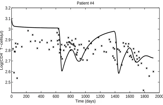
In Figure 1 we depict the log-scaled longitudinal observations (data) on the number of CD4+T-cells,{𝑦
𝑖}, and the model output evaluated at the estimate (the nominal parameter
values described above),𝑧(𝑡𝑖; ˆ𝜃𝑂𝐿𝑆), for Patient #4 in [1, 4].
Given the vector
𝜃= (𝜃1, 𝜃2)∈ℝ28,
parti-0 200 400 600 800 1000 1200 1400 1600 1800 2000 2.5
2.6 2.7 2.8 2.9 3 3.1 3.2
Time (days)
Log(CD4
+ T−cells/
μ
l)
Patient #4
Figure 1: Log-scaled data {𝑦𝑖} of Patient 4 CD4+ T-cells (represented as ‘x’), and model
output 𝑧(𝑡; ˆ𝜃𝑂𝐿𝑆) (represented by the solid curve) evaluated at parameter estimates
ob-tained in [1, 4].
tioning into fixed and active (those to possibly be estimated) parameters. It is assumed the following entries are always fixed at known values provided in [1, 4]: 𝑥0
3,𝑥04,𝑥06,𝜌1, and 𝜌2. In other words, we will calculate sub-vectors from theℝ23 vector
𝑞= (𝑥0
1, 𝑥02, 𝑥05, 𝜆1, 𝑑1, 𝜖1, 𝑘1, 𝜆2, 𝑑2, 𝑓, 𝑘2, 𝛿, 𝑚1, 𝑚2, 𝜖2, 𝑁𝑇, 𝑐, 𝜆𝐸, 𝑏𝐸, 𝐾𝑏, 𝑑𝐸, 𝐾𝑑, 𝛿𝐸). (22)
For every fixed value of 𝑝, such that 𝑝= 2,3, . . . ,22, there are two partitions of interest: one with𝑝active parameters, and the other one with 23−𝑝fixed parameters. For example, when𝑝= 22 one of twenty three possible partitions is the following: fix 𝑥0
1 and consider
(𝑥02, 𝑥05, 𝜆1, 𝑑1, 𝜖1, 𝑘1, 𝜆2, 𝑑2, 𝑓, 𝑘2, 𝛿, 𝑚1, 𝑚2, 𝜖2, 𝑁𝑇, 𝑐, 𝜆𝐸, 𝑏𝐸, 𝐾𝑏, 𝑑𝐸, 𝐾𝑑, 𝛿𝐸)𝑇 ∈ℝ22,
as a vector with active parameters. In the implementation of this subset selection algorithm, we carry out the calculation of all possible vectors by using binary matrices with twenty eight columns, such that every row has zeros for entries that are fixed, and ones for those that are active. In the example above, the binary row is (recall that𝑥0
3,𝑥04,𝑥06,𝜌1, and 𝜌2 are fixed throughout)
(0,1,0,0,1,0,1,1,1,1,1,1,1,1,1,1,1,1,1,1,0,0,1,1,1,1,1,1).
For a fixed value of 𝑝the set
collects all the possible active parameter vectors inℝ𝑝.
We define the set
Θ𝑝 ={𝜃∣𝜃∈ 𝒮𝑝 ⊂ℝ𝑝, rank(𝜒(𝜃)) =𝑝}, (24)
where𝜒(𝜃) denotes the 𝑛×𝑝 sensitivity matrix. By construction, the elements of Θ𝑝 are
parameter vectors that give sensitivity matrices with independent columns.
The next step in the selection procedure involves the calculation of standard errors (uncertainty quantification) using the asymptotic theory (see (20)). For every 𝜃∈Θ𝑝, we
define a vector ofcoefficients of variation 𝜈(𝜃)∈ℝ𝑝 such that for each 𝑖= 1, . . . , 𝑝,
𝜈𝑖(𝜃) = √
(Σ(𝜃))𝑖𝑖
𝜃𝑖 ,
and
Σ(𝜃) =𝜎02[𝜒(𝜃)𝑇𝜒(𝜃)]−1 ∈ℝ𝑝×𝑝.
The components of the vector𝜈(𝜃) are the ratios of each standard error for a parameter to the corresponding nominal parameter value. These ratios are dimensionless numbers warrenting comparison even when parameters have considerably different scales and units (e.g., 𝑁𝑇 is on the order of 101, while 𝑘1 is on the order of 10−6). We then define the selection score as
𝛼(𝜃) =∣𝜈(𝜃)∣,
where∣ ⋅ ∣ is the norm inℝ𝑝. A selection score 𝛼(𝜃) near zero indicates lower uncertainty
possibilities in the estimation, while large values of𝛼(𝜃) suggest that one could expect to find substantial uncertainty in at least some of the components of the estimates in any parameter estimation attempt.
We summarize the steps of the algorithm as follows:
1. All possible active vectors. For a fixed value of𝑝= 2, . . . ,22, fix 23−𝑝parameters to nominal values, and then calculate the set𝒮𝑝, which collects all the possible active
parameter vectors in ℝ𝑝:
𝒮𝑝 ={𝜃∈ℝ𝑝∣𝜃 is a sub-vector of𝑞∈ℝ23defined in equation (22)}.
2. Full rank test. Calculate the set Θ𝑝 as follows
Θ𝑝 ={𝜃∣𝜃∈ 𝒮𝑝⊂ℝ𝑝, rank(𝜒(𝜃)) =𝑝}.
3. Standard error test. For every𝜃∈Θ𝑝 calculate a vector of coefficients of variation
𝜈(𝜃)∈ℝ𝑝 by
𝜈𝑖(𝜃) = √
(Σ(𝜃))𝑖𝑖
𝜃𝑖 ,
for𝑖= 1, . . . , 𝑝, and Σ(𝜃) = 𝜎2
4 Results and Discussion
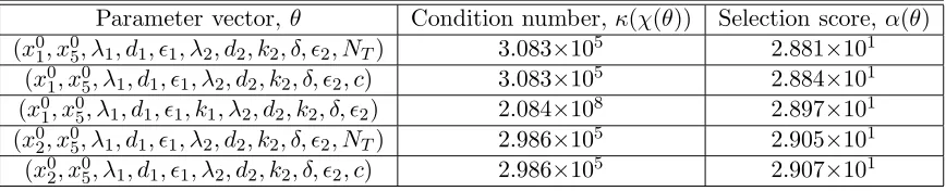
Results of the subset selection algorithm with the HIV model of Section 1.1 are given in Table 2. Parameter vectors, condition numbers (ratio of largest to smallest singular value [40]), and values of the selection score are displayed for𝑝= 11. The third column of Table 2 displays selection score values from smallest (top) to largest (bottom). For the sake of clarity we only display five out of one million parameter vectors chosen by the selection algorithm. The selection score values range from 2.813×101 to 2.488×10⁵ for the one million parameter vectors selected when𝑝= 11.
Table 2: Parameter vectors obtained with subset selection algorithm for𝑝= 11. For each parameter vector𝜃∈Θ𝑝the sensitivity matrix condition number𝜅(𝜒(𝜃)), and the selection
score𝛼(𝜃) are displayed.
Parameter vector,𝜃 Condition number,𝜅(𝜒(𝜃)) Selection score,𝛼(𝜃) (𝑥0
1, 𝑥05, 𝜆1, 𝑑1, 𝜖1, 𝜆2, 𝑑2, 𝑘2, 𝛿, 𝜖2, 𝑁𝑇) 3.083×10⁵ 2.881×101
(𝑥0
1, 𝑥05, 𝜆1, 𝑑1, 𝜖1, 𝜆2, 𝑑2, 𝑘2, 𝛿, 𝜖2, 𝑐) 3.083×10⁵ 2.884×101 (𝑥0
1, 𝑥05, 𝜆1, 𝑑1, 𝜖1, 𝑘1, 𝜆2, 𝑑2, 𝑘2, 𝛿, 𝜖2) 2.084×10⁸ 2.897×101 (𝑥0
2, 𝑥05, 𝜆1, 𝑑1, 𝜖1, 𝜆2, 𝑑2, 𝑘2, 𝛿, 𝜖2, 𝑁𝑇) 2.986×10⁵ 2.905×101
(𝑥0
2, 𝑥05, 𝜆1, 𝑑1, 𝜖1, 𝜆2, 𝑑2, 𝑘2, 𝛿, 𝜖2, 𝑐) 2.986×10⁵ 2.907×101
In [1, 4], the authors estimate the parameter vector
𝜃= (𝑥01, 𝑥02, 𝑥05, 𝜆1, 𝑑1, 𝜖1, 𝑘1, 𝜖2, 𝑁𝑇, 𝑐, 𝑏𝐸)∈ℝ11.
The selection algorithm chooses most of these parameters. For instance, the sub-vector (𝑥0
5, 𝜆1, 𝑑1, 𝜖1, 𝜖2) appears in every one of the top five parameter vectors displayed in Table 2. However, the sub-vector (𝑥0
1, 𝑥02, 𝑥05) along with 𝑏𝐸 are never chosen among the top five
parameter vectors. Even so, use of the subset selection algorithm discussed here (had it been available) might have proved valuable in the efforts reported in [1, 4].
3 4 5 6 7 8 9 10 11 12 13 14 15 16 17 18 0
2000 4000 6000 8000 10000 12000
Number of parameters
Selection score
(a)
3 4 5 6 7 8 9 10 11 12 13 14 15 16 17 18
10−1 100 101 102 103 104 105
Number of parameters
Ln(Selection score)
(b)
101 102 103 104 105 106 107 108 109 10−1
100 101 102 103 104 105
Sensitivity matrix condition number
Selection score
p=5
p=18
Figure 3: Selection score 𝛼(𝜃) versus condition number 𝜅(𝜒(𝜃)), where𝜃 ∈ ℝ𝑝, for 𝑝 = 5
(circles) and 𝑝= 18 (triangles). Both axes are in logarithmic scale. The smallest hundred values of the selection score are depicted for each value of𝑝.
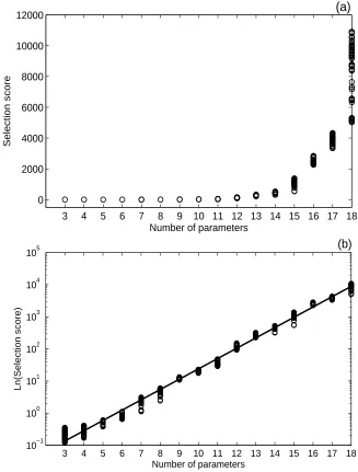
with the number of parameters to be estimated. More precisely, for 3≤𝑝≤18, we find
𝛼≡𝛼(𝑝) =𝐶𝑒0.75𝑝, (25)
where𝐶 = 8.52×10⁻⁴.
In Figure 3 we graph (in logarithmic scales) the smallest one hundred selection score values𝛼(𝜃) versus the sensitivity matrix condition number 𝜅(𝜒(𝜃)), with 𝜃∈ℝ𝑝, for𝑝= 5
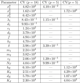
In Table 3 we examine the effect that removing parameters from an estimation has in uncertainty quantification. The coefficient of variation (CV) is defined as the ratio of the standard error to the estimate for each parameter. In Table 3 three cases are considered: 𝑝 = 18, where 𝜃 = (𝑥0
1, 𝑥02, 𝑥05, 𝜆1, 𝑑1, 𝜖1, 𝑑2, 𝑓, 𝑘2, 𝛿, 𝑚1, 𝑚2, 𝜖2, 𝑁𝑇, 𝑏𝐸, 𝐾𝑏, 𝑑𝐸, 𝐾𝑑); 𝑝 = 5,
where𝜃= (𝑥0
1, 𝜆1, 𝛿, 𝜖2, 𝑁𝑇); and𝑝= 5, where 𝜃= (𝑥02, 𝑏𝐸, 𝐾𝑏, 𝑑𝐸, 𝐾𝑑).
There are consistent improvements in uncertainty quantification, with CV dropping as much as four orders of magnitude. For instance, by comparing the second and third columns of Table 3, one sees the reduction of CV for𝜆1, going from 8.430×10⁻¹to 1.150×10⁻¹, im-plies the standard error is 84% of the estimate for𝑝= 18, while it reduces to 11% of the esti-mate when𝑝= 5. For the parameter𝑁𝑇, it is observed that the standard error reduces from
being 40000% to 10% of the estimate. A similar remarkable improvement is also seen for𝑥0 1, with a standard error equal to 50000% of the estimate for𝑝= 18, dropping to 4% of the esti-mate for𝑝= 5. The improvement in uncertainty quantification is related to going from the upper right corner of Figure 3 into the lower left corner. On one hand, the condition number and selection score for 𝜃 = (𝑥0
1, 𝑥02, 𝑥05, 𝜆1, 𝑑1, 𝜖1, 𝑑2, 𝑓, 𝑘2, 𝛿, 𝑚1, 𝑚2, 𝜖2, 𝑁𝑇, 𝑏𝐸, 𝐾𝑏, 𝑑𝐸, 𝐾𝑑),
are 7.518×10⁸ and 1.025×10⁵, respectively. On the other hand, the condition number and selection score for𝜃= (𝑥0
1, 𝜆1, 𝛿, 𝜖2, 𝑁𝑇) are 8.383×101 and 3.990×10⁻¹, respectively.
The fourth column of Table 3 is evidence that simply reducing the number of param-eters (e.g. from 𝑝 = 18 to 𝑝 = 5) is not sufficient to guarantee reasonable improvements in uncertainty quantification, even though equation (25) establishes an exponential rela-tionship between the norm of the vector of coefficients of variation and the number of parameters. When comparing the second and fourth column of Table 3, the best improve-ment in uncertainty quantification is observed for𝑥0
Table 3: Coefficient of variation (CV), defined as the ratio of standard error divided by estimate, for three parameter vectors.
Parameter CV (𝑝= 18) CV (𝑝= 5) CV(𝑝= 5) 𝑥0
1 4.82×10² 4.10×10⁻² —
𝑥0
2 1.62×10⁴ — 1.72×100
𝑥0
5 6.42×10³ — —
𝜆1 8.43×10⁻¹ 1.15×10⁻¹ —
𝑑1 9.93×10⁻¹ — —
𝜖1 1.24×10² — —
𝑑2 3.79×101 — —
𝑓 4.94×10² — —
𝑘2 4.70×101 — —
𝛿 3.98×10² 3.39×10⁻¹ —
𝑚1 2.24×10⁴ — —
𝑚2 3.82×10⁴ — —
𝜖2 2.06×10² 1.39×10⁻¹ — 𝑁𝑇 4.04×10² 9.99×10⁻² —
𝑏𝐸 6.10×10⁴ — 1.12×10⁴
𝐾𝑏 2.51×10⁴ — 4.29×10³
𝑑𝐸 5.79×10⁴ — 1.07×10⁴
5 Concluding Remarks
As we have noted, inverse problems for complex system models containing a large number of parameters are difficult. There is great need for quantitative methods to assist in posing inverse problems that will be well formulated in the sense of the ability to provide parameter estimates with quantifiable small uncertainty estimates. We have introduced and illustrated use of such an algorithm that requires prior local information about ranges of admissible parameter values and initial values of interest along with a minimum of information (an estimate of the variance) on the error in the observation process to be used with the inverse problem. These are needed in order to implement the sensitivity/Fisher matrix based algorithm. The rank of the sensitivity matrix and, consequently, the conditioning of the Fisher information matrix, play an important role in the results obtained with OLS inverse problems. As seen in equation (21), the measurement error is amplified in the estimator as the ill-conditioning of the Fisher information matrix increases.
From our computations as summarized in this note, we may conclude that the proposed selection score, which involves uncertainty quantification, grows exponentially with the number of parameters (see Figure 2 and equation (25)). However, as we have observed, improvements in uncertainty quantification are obtained not only by reducing the number of parameters, but also by carefully selecting key parameters from the inverse problem for a given number of parameters.
Because the ability to estimate a model parameter is fundamentally related to sensitivity of the model with respect to the parameter, and because sensitivity is a local concept, we observe that the pursuit of a global algorithm to use in formulating parameter estimation or inverse problems is most likely a quest that will go unfulfilled.
Acknowledgements
This research was supported in part by Grant Number R01AI071915-07 from the National Institute of Allergy and Infectious Diseases and in part by the Air Force Office of Scientific Research under grant number FA9550-09-1-0226. A. C.-A. carried portions of this work while visiting the Statistical and Applied Mathematical Sciences Institute, which is funded by the National Science Foundation under Grant DMS-0635449. The content is solely the responsibility of the authors and does not necessarily represent the official views of the NIAID, the NIH, the AFOSR, or the NSF.
References
[2] B.M. Adams, H.T. Banks, M. Davidian, H. Kwon, H.T. Tran, S.N. Wynne and E.S. Rosenberg, HIV dynamics: modeling, data analysis, and optimal treatment protocols, J. Comp. and Appl. Math.,184 (2005), 10–49.
[3] B.M. Adams, H.T. Banks, H.T. Tran and H. Kwon, Dynamic multidrug therapies for HIV: optimal and STI control approaches,Math. Biosci. and Engr.,1(2004), 223–241. [4] B.M. Adams, H.T. Banks, M. Davidian and E.S. Rosenberg, Model fitting and predic-tion with HIV treatment interruppredic-tion data, CRSC-TR05-40, NCSU, October, 2005; Bull. Math. Biol.,69 (2007), 563–584.
[5] D.T. Anh, M.P. Bonnet, G. Vachaud, C.V. Minh, N. Prieur, L.V. Duc and L.L. Anh, Biochemical modeling of the Nhue River (Hanoi, Vitenam): practical identifiability analysis and parameter estimation, Ecol. Model.,193 (2006), 182–204.
[6] K.J. Astrom and P. Eykhoff, System identification–A survey, Automatica, 7 (1971), 123–162.
[7] H.T. Banks, M. Davidian, J.R. Samuels and K.L. Sutton, An inverse problem statis-tical methodology summary, Center for Research in Scientific Computation Technical Report CRSC-TR08-1, NCSU, January, 2008; in Mathematical and Statistical Esti-mation Approaches in Epidemiology, (eds. G. Chowell, et. al.), Springer, New York, 2009, pp. 249–302.
[8] H.T. Banks, M. Davidian, S. Hu, G. M Kepler and E. S. Rosenberg, Modeling HIV immune response and validation with clinical data, CRSC-TR07-09, March, 2007; J. Biological Dynamics,2 (2008), 357–385.
[9] H.T. Banks, S. Dediu and S.E. Ernstberger, Sensitivity functions and their uses in inverse problems, CRSC Technical Report, CRSC-TR07-12, NCSU, July, 2007; J. Inverse and Ill-posed Problems,15 (2007), 683–708.
[10] H.T. Banks, S. Dediu, S.L. Ernstberger and F. Kappel, Generalized sensitivities and optimal experimental design, Center for Research in Scientific Computation Technical Report CRSC-TR08-12, NCSU, September, 2008, Revised, November, 2009;J. Inverse and Ill-posed Problems,18(2010), 25–83.
[11] H. T. Banks, S. L. Ernstberger and S. L.Grove, Standard errors and confidence inter-vals in inverse problems: sensitivity and associated pitfalls, J. Inverse and Ill-posed Problems,15(2007), 1–18.
[13] H. T. Banks and B. G. Fitzpatrick, Statistical methods for model comparison in pa-rameter estimation problems for distributed systems, CAMS Tech. Rep. 89-4, Septem-ber, 1989, University of Southern California; J. Math. Biol.,28(1990), 501–527. [14] H.T. Banks, K. Holm and D. Robbins, Standard error computations for uncertainty
quantification in inverse problems: Asymptotic theory vs. bootstrapping, Center for Research in Scientific Computation Technical Report CRSC-TR09-13, NCSU, June, 2009; Revised August, 2009; Arabian Journal for Science and Engineering: Mathe-matics (AJSE-MatheMathe-matics), submitted.
[15] H.T. Banks and J.R. Samuels, Jr., Detection of cardiac occlusions using viscoelastic wave propagation, CRSC-TR08-23, December, 2008; Advances in Applied Mathemat-ics and MechanMathemat-ics, 1 (2009), 1–28.
[16] J. J. Batzel, F. Kappel, D. Schneditz and H. T. Tran,Cardiovascular and Respiratory Systems: Modeling, Analysis and Control, Frontiers in Applied Mathematics FR34, SIAM, Philadelphia, 2006.
[17] E.J. Bedrick and C.L. Tsai, Model selection for multivariate regression in small sam-ples, Biometrics,50(1994), 226–231.
[18] R. Bellman and K.M. Astrom, On structural identifiability, Math. Biosci., 7 (1970), 329–339.
[19] R. Bellman and R. Kalaba, Quasilinearization and Nonlinear Boundry Value Prob-lems, American Elsevier, New York, 1965.
[20] S. Bonhoeffer, M. Rembiszewski, G.M. Ortiz and D.F. Nixon, Risks and benefits of structured antiretroviral drug therapy interruptions in HIV-1 infection, AIDS,14 (2000), 2313–2322.
[21] H. Bozdogan, Model selection and Akaike’s Information Criterion (AIC): The general theory and its analytical extensions, Psychometrika,52(1987), 345–370.
[22] H. Bozdogan, Akaike’s Information Criterion and recent developments in information complexity, Journal of Mathematical Psychology,44(2000), 62–91.
[23] M. Burth, G.C. Verghese and M. V´elez-Reyes, Subset selection for improved parameter estimation in on-line identification of a synchronous generator, IEEE T. Power Syst., 14 (1999), 218–225.
[25] K. P. Burnham and D.R. Anderson, Multimodel inference: Understanding AIC and BIC in model selection, Sociological Methods and Research, 33(2004), 261–304. [26] D.S. Callaway and A.S. Perelson, HIV-1 infection and low steady state viral loads,
Bulletin of Mathematical Biology,64(2001) 29–64.
[27] A. Cintr´on-Arias, C. Castillo-Ch´avez, L.M.A. Bettencourt, A.L. Lloyd and H.T. Banks, The estimation of the effective reproductive number from disease outbreak data, Tech Rep CRSC-TR08-08, NCSU, April, 2008; Math. Biosci. Engr., 6 (2009), 261–283.
[28] A. Cintr´on-Arias, H.T. Banks, A. Capaldi and A.L. Lloyd, A sensitivity matrix based methodology for inverse problem formulation, Tech Rep CRSC-TR09, NCSU, April, 2009; J. Inverse and Ill-posed Problems, 17(2009), 545–564.
[29] C. Cobelli and J. J. DiStefano III, Parameter and structural identifiability concepts and ambiguities: a critical review and analysis, Am. J. Physiol.239 (1980), R7–R24. [30] M. Davidian and D.M. Giltinan, Nonlinear Models for Repeated Measurement Data,
Chapman & Hall, Boca Raton, 1995.
[31] B. Efron and R.J. Tibshirani, An Introduction to the Bootstrap, Chapman & Hall / CRC, Boca Raton, 1998.
[32] H.W. Engl, C. Flamm, P. K¨ugler, J. Lu, S. M¨uller and P. Schuster, Inverse problems in system biology, Inverse Problems,25(2009), 123014(51pp).
[33] P. Eykhoff, System Identification: Parameter and State Estimation, Wiley & Sons, New York, 1974.
[34] M. Eslami, Theory of Sensitivity in Dynamic Systems: an Introduction, Springer-Verlag, New York, NY, 1994.
[35] N.D. Evans, L.J. White, M.J. Chapman, K.R. Godfrey and M.J. Chappell, The struc-tural identifiability of the susceptible infected recovered model with seasonal forcing, Math. Biosci.,194 (2005), 175–197.
[36] M. Fink, myAD: fast automatic differentiation code in MATLAB, 2006; http://gosh.gmxhome.de/
[37] M. Fink, A. Attarian and H. Tran, Subset selection for parameter estimation in an HIV model,Proc. Applied Math. and Mechanics,7 (2008), 1121501–1121502.
[39] K. Glover and J.C. Willems, Parametrizations of linear dynamical systems: Canonical forms and identifiability, IEEE Trans. Automat. Contr.,AC-19 (1974), 640–645. [40] G.H. Golub and C.F. Van Loan, Matrix Computations, Johns Hopkins University
Press, Baltimore, 1996.
[41] C.M. Hurvich and C.L. Tsai, Regression and time series model selection in small samples, Biometrika,76(1989), 297–307.
[42] A. Holmberg, On the practical identifiability of microbial growth models incorporating Michaelis-Menten type nonlinearities, Math. Biosci.,62(1982), 23–43.
[43] L.E. Jones and A.S. Perelson, Opportunistic infection as a cause of transient viremia in chronically infected HIV patients under treatment with HAART,Bull. Math. Biol., 67 (2005), 1227–1251.
[44] R.E Kalman, Mathematical description of linear dynamical systems,SIAM J. Control, 1 (1963), 152–192.
[45] D. G. Luenberger, Optimization by Vector Space Methods, John Wiley & Sons, New York, NY, 1969.
[46] A.K. Mehra and D.G. Lainiotis, System Identification, Academic Press, New York, 1976.
[47] I.M. Navon, Practical and theoretical aspects of adjoint parameter estimation and identifiability in meteorology and oceanography, Dyn. Atmospheres and Oceans, 27 (1997), 55–79.
[48] P. Nelson, N. Smith, S. Cuipe, W. Zou, G. S. Omenn and M. Pietropaolo, Modeling dynamic changes in type 1 diabetes progression: Quantifying 𝛽-cell variation after the appearance of islet-specific autoimmune responses,Math. Biosci. Eng., 6 (2009), 753–778.
[49] M.A. Nowak and C.R.M. Bangham, Population dynamics of immune responses to persistent viruses, Science,272(1996), 74–79.
[50] J. T. Ottesen, M. S. Olufsen and J. K. Larsen,Applied Mathematical Models in Hu-man Physiology, Monographs on Mathematical Modeling and Computation, MM09, SIAM, Philadelphia, 2004.
[51] A.S. Perelson and P.W. Nelson, Mathematical analysis of HIV-1 dynamics in vivo, SIAM Review,41(1999),3–44.
[53] A.P. Sage and J.L. Melsa, System Identification, Academic Press, New York, 1971. [54] G.A.F. Seber and C.J. Wild, Nonlinear Regression, John Wiley & Sons, Chichester,
2003.
[55] J. Shao and D. Tu, The Jackknife and Bootstrap, Springer-Verlag, New York, 1995. [56] K. Thomaseth and C. Cobelli, Generalized sensitivity functions in physiological system
identification, Ann. Biomed. Eng.,27(5) (1999), 607 – 616.
[57] D. Wodarz and M.A. Nowak, Specific therapy regimes could lead to long-term immuno-logical control of HIV,Proc. National Academy of Sciences,96 (1999), 14464–14469. [58] L.J. White, N.D. Evans, T.J.G.M. Lam, Y.H. Schukken, G.F. Medley, K.R. Godfrey
and M.J. Chappell, The structural identifiability and parameter estimation of a mul-tispecies model for the transmission of mastitis in diary cows, Math. Biosci., 174 (2001), 77–90.
[59] H. Wu, H. Zhu, H. Miao and A.S. Perelson, Parameter identifiability and estimation of HIV/AIDS dynamics models, Bull. Math. Biol.,70(2008), 785–799.
[60] X. Xia and C.M. Moog, Identifiability of nonlinear systems with application to HIV/AIDS models, IEEE T. Automat. Contr.,48(2003), 330–336.