1
The influence of match phase and field position on collective team behaviour in Australian 2
Rules Football 3
4 5
Authors 6
Jeremy. P. Alexander 1*., Bartholomew Spencer1., Alice J. Sweeting 1, 3., Jocelyn. K. Mara 2., Sam Robertson 1, 3 7
8
Department/Institution
9
1Institute for Health and Sport (IHES) 10
Victoria University,
11
Melbourne VIC, Australia
12 13
2Research Institute for Sport and Exercise 14
University of Canberra
15
Bruce, ACT, 2617, Australia
16
(02) 6201 5111
17 18
3Western Bulldogs Football Club 19
Melbourne, VIC, Australia
20 21
*Corresponding author 22
Email: [email protected] 23
24
Word Count: 3770 25
Number of Figures: 5 26
ABSTRACT 29
30
This study investigated the influence of match phase and field position on collective team 31
behaviour in Australian Rules football (AF). Data from professional male athletes (years 24.4 ± 32
3.7; cm 185.9 ± 7.1; kg 85.4 ± 7.1), were collected via 10 Hz global positioning system (GPS) 33
during a competitive AFL match. Five spatiotemporal metrics (x-axis centroid, y–axis centroid, 34
length, width, and surface area), occupancy maps, and Shannon Entropy (ShannEn) were analysed 35
by match phase (offensive, defensive, and contested) and field position (defensive 50, defensive 36
midfield, forward midfield, and forward 50). A multivariate analysis of variance (MANOVA) 37
revealed that field position had a greater influence on the x-axis centroid comparative to match 38
phase. Conversely, match phase had a greater influence on length, width, and surface area 39
comparative to field position. Occupancy maps revealed that players repositioned behind centre 40
when the ball was in their defensive half and moved forward of centre when the ball was in their 41
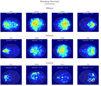
forward half. Shannon Entropy revealed that player movement was more variable during offence 42
and defence (ShannEn = 0.82 – 0.93) compared to contest (ShannEn = 0.68 – 0.79). Spatiotemporal 43
metrics, occupancy maps, and Shannon Entropy may assist in understanding the game style of AF 44
teams. 45
46
Key Words: Performance analysis, Team tactics, Game style 47
INTRODUCTION 49
50
Collective team behaviour in invasion sports refers to how individual players position themselves 51
across a field of play to form an overall group organisation (Rein and Memmert 2016). This 52
behaviour has been used to describe team tactics or game style, whereby repetitive patterns of 53
movement are formed (Sampaio and Macas 2012). Collective team behaviour has become a central 54
component of match analysis (Clemente, Sequeiros et al. 2018) due to its established relationship 55
with performance outcomes (Clemente, Couceiro et al. 2013, Goncalves, Marcelino et al. 2016, 56
Rein and Memmert 2016) and the capability to provide greater context to match events (Lamas, 57
Barrera et al. 2014). 58
Collective team behaviour has typically been defined via spatiotemporal metrics including 59
x-axis centroid, y-axis centroid, length, width, and surface area (Frencken, Lemmink et al. 2011, 60
Clemente, Couceiro et al. 2013, Folgado, Lemmink et al. 2014). The team centroid represents the 61
geometric centre of all players on the field, which can be assessed in both the x-axis and y-axis, 62
team length and width describes the distance between the two players furthest apart along the pitch 63
and across the pitch respectively, and the team surface area signifies the region that encompasses 64
all players across a field of play (Bartlett, Button et al. 2012). More recently, studies have 65
visualised occupancy maps or heat maps and combined them with a measure of entropy to 66
determine the variability of player movement (Couceiro, Clemente et al. 2014, Silva, Aguiar et al. 67
2014, Clemente, Sequeiros et al. 2018). To provide additional context to the understanding of 68
collective behaviour, investigations have been separated into various phases of match play, such 69
as offence and defence (Castellano, Álvarez et al. 2013, Clemente, Couceiro et al. 2013, 70
Research in football has considered the x-axis centroid and occupancy maps to suggest 72
teams may be more attacking by positioning players higher up the field in both offence and defence 73
during home matches compared to away matches (Lucey, Oliver et al. 2013, Bialkowski, Lucey et 74
al. 2014). This behaviour may be associated with an increased possession in the forward third and 75
a greater number of shots on goal (Lucey, Oliver et al. 2013, Bialkowski, Lucey et al. 2014). 76
Irrespective of match location, a conservative approach is generally taken, with the team x-axis 77
centroid located in their defensive half (Clemente, Couceiro et al. 2013). Investigations in football 78
have used the length, width, and surface area to propose that whilst defending, teams will aim to 79
compress the field of play by decreasing the area in which attacking players can operate (Vilar, 80
Araújo et al. 2013). Increasing the number of defensive players surrounding an attacking team 81
taking a shot at goal is associated with a concomitant decrease in successful scoring attempts 82
(Ensum, Pollard et al. 2004, Wright, Atkins et al. 2011). Conversely, when teams are in offence 83
they will attempt to spread the opposing defence to create more space (Castellano and 84
Casamichana 2015). Defending players are then compelled to either restrict the impact of these 85
players or hold their position to protect space closer towards their goal (Vilar, Araújo et al. 2013). 86
Higher-ranking teams in football may therefore be more effective at accomplishing this as they 87
commonly produce greater values of length, width, and playing space compared to their lower-88
ranked counterparts (Castellano, Álvarez et al. 2013). 89
Due to the continuous nature of invasion sports, it is difficult to associate discrete parts of 90
collective team behaviour with a certain type of play (Lucey, Oliver et al. 2013). Specifically, it 91
may be somewhat simplistic to assign specific movement behaviour to a particular tactic or game 92
style, as a team’s movement behaviour is constantly influenced by emerging aspects of match play 93
preconceived team tactic or game style but rather an adaption to the general state of play (Rein and 95
Memmert 2016). Thus, to gain a more comprehensive representation of team tactics or game style, 96
researchers should account for contextual variables, such as match phase and field position 97
(Castellano, Álvarez et al. 2013, Clemente, Couceiro et al. 2013, Alexander, Spencer et al. 2018). 98
Research into collective team behaviour in Australian Football (AF) also remains largely absent, 99
with only one study reported to date (Alexander, Spencer et al. 2018). 100
Australian Football is an invasion sport where teams compete on an oval shaped field 101
(length = ~160 m, width = ~130 m). The match is separated into four quarters, contested by 22 102
players per team, with 18 on the field and 4 on an interchange bench (Gray and Jenkins 2010). 103
Initial research in AF identified that teams display large variations in overall positioning 104
throughout a match that may be influenced by the position of the ball (Alexander, Spencer et al. 105
2018). Therefore, field position of the ball may influence collective team behaviour (Alexander, 106
Spencer et al. 2018). However, the extent to which collective team behaviour is influenced by 107
match phase in relation to field position is yet to be investigated. 108
Determining collective team behaviour whilst accounting for contextual variables may 109
provide a greater understanding of team tactics or game style. Therefore, this study investigated 110
the influence of match phase and field position on collective team behaviour in AF. 111
112
METHODS 113
114
Data were collected from 22 male professional AF players (years 24.4 ± 3.7; cm 185.9 ± 7.1; kg 115
85.4 ± 7.1), recruited from a single team in the Australian Football League (AFL) competition. 116
information about the requirements of the study via verbal and written communication, and 118
provided their written consent to participate. The University Ethics Committee approved the study. 119
The match took place on an oval shaped ground using dimensions 159.5 m x 128.8 m 120
(length x width) with four 20-min quarters. Spatiotemporal data for all participants were collected 121
using 10 Hz GPS devices (Catapult Optimeye S5, Catapult Innovations, Melbourne, Australia). 122
The devices were housed in a sewn pocket in the jersey that is located on the upper back. The 123
number of GPS satellites were greater than 8 packets per second, which ensured adequate signal 124
quality (Corbett, Sweeting et al. 2017). 125
Spatiotemporal data was exported in raw 10 Hz format. Each file contained a global time 126
stamp and calibrated location (x- and y- location). Match phase was determined via which team 127
had possession of the ball (offensive, defensive or contest). The offensive phase was recorded 128
when a team first gained possession of the ball and maintained it for at least a second and ended 129
when the opposing team gained possession of the ball for at least a second or there was a stoppage 130
in play. For example, the team scored or the ball went out of bounds (Yue, Broich et al. 2008). 131
Using the same conditions, the defensive phase was recorded when the opposing team had 132
possession of the ball (Yue, Broich et al. 2008). If neither team had possession of the ball, for 133
example, when the officiating umpire returned the ball to play, the phase was considered to be in 134
contest until a team gained possession of the ball for at least one second. All periods where the 135
ball was out of play, for example, when there was a break between periods of play, celebration 136
after goals, were excluded from the investigation. Field position of the ball was separated into four 137
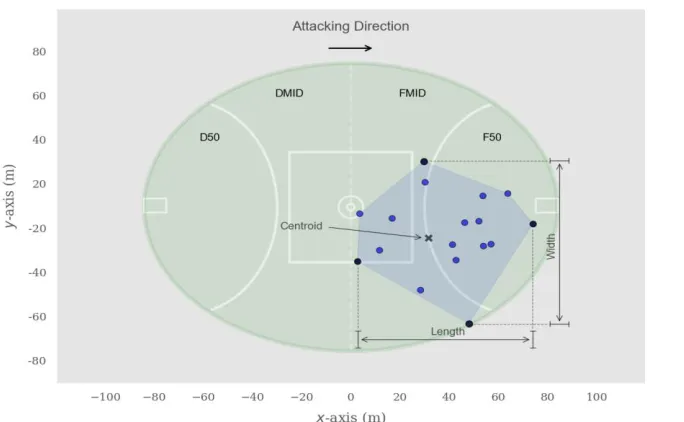
zones (defensive 50; D50, defensive mid; DMID, forward mid; FMID, forward 50; F50) by the 138
two 50 m arcs and the centre of the ground (see Figure 1). The centre of the ground was signified 139
nearest second by a commercial statistical provider (Champion Data Pty Ltd, Melbourne, 141
Australia). Previous investigations have assessed the validity and reliability of similar match 142
events (Robertson, Gupta et al. 2016). Positional data was then synchronised with match phase 143
and field position data using the respective global timestamps. This was established using the 144
initial point when the two widest players on the field converged from a stationary position prior to 145
start of each quarter. 146
147
148
Figure 1: Four field position zones and spatiotemporal metrics including centroid, length, width, 149
and surface area. 150
151
Five spatiotemporal metrics (Figure 1) were derived from the data to describe collective 152
team behaviour. Team centroid was calculated as the mean (x, y) position of all players on the field 153
were the distance in the x-axis centroid (m) and the distance in the y-axis centroid (m) (Frencken, 155
Lemmink et al. 2011). The team surface area was calculated as the total space (m) covered by a 156
single team (Frencken, Lemmink et al. 2011). Team length was measured as the distance between 157
the most forward and most backward player in the x-axis (m) and team width was defined as the 158
distance between the two most lateral players on the ground in the y-axis (m) (Frencken, Lemmink 159
et al. 2011). Variability of player movement was visualised via occupancy maps (Couceiro, 160
Clemente et al. 2014, Silva, Aguiar et al. 2014), which represent the density of players across a 161
given area (Silva, Aguiar et al. 2014). The occupancy maps were combined with Shannon Entropy 162
(ShannEn) to provide an enhanced understanding of team movement variability. To calculate 163
ShannEn, the field of play was quantised into bins of equal size (1m2) to provide adequate spatial 164
resolution (Couceiro, Clemente et al. 2014). The total count from each bin was used to determine 165
the total time spent in each bin. A probability distribution of the total time spent in each bin was 166
then used to determine the variability of a player being located in a specific bin. Both the heat 167
maps and ShannEn values were normalised to total time spent in each position on the field for each 168
match phase. Synchronisation and analysis were undertaken using the computational package 169
Python version 3.2 with Spyder, which is part of the Anaconda software suite (www.python.org). 170
171
Statistical Analyses 172
Comparison of team x-axis centroid, y-axis centroid, length, width, and surface area were assessed 173
between match phase (3 levels: Offence, Defence, Contest) and field position (4 levels: D50, 174
DMID, FMID, F50), via a multivariate analysis of variance (MANOVA). Homogeneity was 175
analysed using the Levene Test, which resulted in a lack of uniformity between match phase and 176
number of samples is in each group was essentially equal (Vincent 1999). Due to the non-178
homogeneity of the time series data, the Central Limit Theorem was considered, which allowed 179
the assumption of normality to be made (Akritas 2004). Effect sizes were determined by 180
calculating partial eta-squared (𝜂𝑝2) and was considered as small (𝜂𝑝2< .06), moderate (𝜂𝑝2> .06 𝜂𝑝2
181
< .15) or large (𝜂𝑝2 ≥ .15) (Cohen 1988). Significant p values reported are < .001 unless otherwise
182
stated. These calculations were determined using SPSS, v21.0; Inc., Armonk, NY, USA). Using 183
Shannon Entropy S, the probability p (i) of finding a player in bin i was measured via quantising 184
the field into n bins. Entropy was then normalised N to total match time spent in each position on 185
the field for each phase of play to return a relative number between 0 and 1. 186
187
𝑆 (%) = − ∑ 𝑝 (𝑖) log 𝑝 (𝑖) log 𝑁 𝑛−1
𝑖=0
188
189
A low ShannEn (near 0) suggests the variability of player movement is low (Couceiro, Clemente 190
et al. 2014). A high ShannEn (near 1) indicates the variability of player movement is high 191
(Couceiro, Clemente et al. 2014). These calculations were completed using the computational 192
package Python version 3.2 with Spyder, which is part of the Anaconda software suite 193
(www.python.org). 194
195
RESULTS 196
197
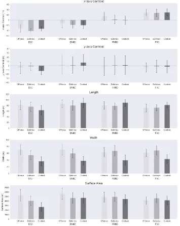
Total differences between match phase and field position for each spatiotemporal metric are 198
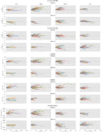
match phase are represented in Figure 3, while the distribution of these sequences are displayed in 200
Figure 4. Heat maps and ShannEn values displaying player movement variability between match 201
phase and field position are presented in Figure 5. The team observed in this study won the game 202
109 – 38. 203
Overall, field position had a greater influence on the x-axis centroid (𝜂𝑝2 = .41) when
204
compared to match phase. Although, match phase had a greater influence on length (𝜂𝑝2 = .06),
205
width (𝜂𝑝2 = .27), and surface area (𝜂𝑝2 = .14) when compared to field position. The x-axis centroid
206
in the D50 was further behind centre when compared to the DMID (-10.7; 95% CI -11.2 – -10.2), 207
FMID (-35.3; 95% CI -35.7 – -34.9) and the F50 (-48.1; 95% CI -48.6 – -47.7). The x-axis centroid 208
in the DMID was also recorded further behind the FMID 24.6; 95% CI -25.0 – -24.1) and F50 (-209
37.4; 95% CI -37.9 – -37.0), while the x-axis centroid in the FMID was recorded forward of centre 210
it was still behind the F50 (-12.9; 95% CI -13.3 – -12.5). Length was greater during the DMID 211
when compared to the D50 (22.9; 95% CI 22.3 – 23.6) and F50 (22.9; 95% CI 22.3 – 23.6). Length 212
in the FMID was also greater than the D50 (8.1; 95% CI 7.6 – 8.7). Width was reduced in the D50 213
when compared to the DMID (-16.7; 95% CI -17.2 – -16.2), FMID (-10.6; 95% CI -11.0 – -10.2), 214
and F50 (-14.5; 95% CI -14.9 – -14.0). The surface area in the DMID was larger when compared 215
to the D50 (1900.3; 95% CI 1857.9 – 1942.8), FMID (976.4; 95% CI 934.4 – 1018.3), and F50 216
(1054.0; 95% CI 1012.3 – 1095.7). Surface area in the FMID was also larger when compared to 217
the D50 (923.9; 95% CI 885.1 – 962.8) and F50 (77.6; 95% CI 39.6 – 115.7). 218
220
Figure 2: Comparison of mean ± standard deviation between match phase and field position of 221
Between-phase analysis recorded the x-axis centroid higher up the ground during offence when 223
compared to defence (3.6; 95% CI 3.1 – 4.0) and contest (3.3; 95% CI 2.6 – 4.0). Length was 224
greater during offence compared to defence (4.7; 95% CI 4.2 – 5.3), while contest was greater than 225
offence (3.5; 95% CI 2.5 – 4.5) and defence (8.2; 95% CI 7.2 – 9.3). Width was greater during 226
offence when compared to defence (3.3; 95% CI 2.9 – 3.8) and contest (27.9; 95% CI 27.2 – 28.7). 227
Width was also greater during defence compared to contest (24.6; 95% CI 23.8 – 25.4). Surface 228
area was greater during offence compared defence (397.5; 95% CI 359.8 – 435.2) and contest 229
(794.2; 95% CI 727.4 – 861.0). Surface area during defence was also greater than contest (396.8; 230
95% CI 327.8 – 465.8). 231
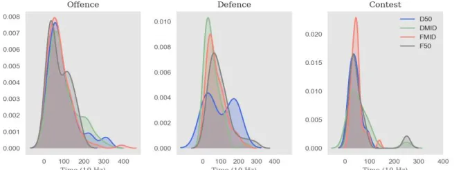
Visual inspection of the distribution plots (Figure 4) displayed similar time duration for 232
offensive and defensive sequences with the majority of playing sequences between 0 – 20 seconds. 233
Total time during contest was reduced with the majority of sequences measuring between 0 – 10 234
236
Figure 3: Comparison of individual instances of spatiotemporal metrics in relation to the 237
239
Figure 4: Between match phase comparison of the distribution of total time for field position 240
241
ShannEn values (Figure 5) were greater during offence and defence compared to contest. 242
Between field position analysis indicated that variability of team movement decreased during 243
defence when in the D50 and in offence when in the F50. ShannEn values were greater during 244
contest when the ball was in the middle of the ground compared to D50 and F50. 245
Commented [ja1]: I could swap the x-axis to seconds for interoperability? It would basically be 0, 10, 20, 30, 40 seconds.
246
Figure 5: Comparison of occupancy maps and ShannEn values for match phase and field position 247
248
DISCUSSION 249
250
This is the first study to investigate the influence of match phase and field position on collective 251
team behaviour in AF. This proof of concept study may be used to provide a complementary 252
framework to add to existing match analyses common in AF. Specifically, the addition of 253
both enhanced insights and context to existing consideration of discrete team and player 255
performance indicators. 256
A predominant finding was field position had a greater influence on the x-axis centroid 257
when compared to phase of play. Conversely, phase of play had a greater influence on length, 258
width, and surface area when compared with field position. Players collectively transitioned closer 259
to their goal when the ball was in their defensive half and pressed higher up the field when the ball 260
was in their forward half. Variation in player movement, as signified by ShannEn, increased 261
through FMID and DMID compared to F50 and D50 and during offence and defence when 262
compared to contest. 263
Overall, the majority of players were positioned close to where the ball was situated. The 264
density of players was more pronounced when the ball was in the D50 or F50 and further amplified 265
when in the contested phase. Length, width, and surface area were also reduced under these 266
circumstances. This type of behaviour may be associated with players trying to reduce the amount 267
of space an opposition can operate in (Vilar, Araújo et al. 2013) and is also representative of AFL 268
rules, whereby no movement restrictions are imparted on players. This behaviour could be 269
beneficial when defending in the D50 as it may be more difficult for the opposing team to achieve 270
an effective shot on goal if an increased number of players are located within this area (Ensum, 271
Pollard et al. 2004, Wright, Atkins et al. 2011). Alternatively, when the ball is located in the F50 272
it may be more difficult for the opposing team to successfully move the ball out of this area if 273
players have setup an effective ‘barrier’ behind the ball. Increased width and variation in player 274
movement throughout the middle of the ground comparative to the F50 and D50 areas may also 275
be somewhat attributed to the oval shaped field dimensions of an AF ground. However, reduced 276
between field position and match phase. Increased variability during offence in the D50, DMID, 278
and FMID could indicate players may be utilising various movement patterns to disrupt opposing 279
defensive structures (Garganta 2009). Reduced movement variation during the contested phase 280
may reflect the inactive period, prior to a change in match phase. The duration of playing sequences 281
during the contested phase was also reduced when compared to offensive and defensive phases. In 282
the present study, while players may produce less movement variation during contest, they are 283
required to be prepared to react when either team gains possession of the ball. 284
Studies investigating the physical movement output of team sport athletes through the 285
duration of time are ubiquitous (Brewer, Dawson et al. 2010, Wisbey, Montgomery et al. 2010, 286
Dwyer and Gabbett 2012). However, there is limited research on the duration of time with respect 287
to collective team behaviour. Findings from the present study indicate the time duration of playing 288
sequences before a change in field position are generally between 0 and 20 seconds for offensive 289
and defensive phases and 0 to 10 seconds for the contested phase. The combination of 290
spatiotemporal metrics, heat maps, and entropy measures may assist in measuring particular 291
collective team behaviour, which can be used to design more representative training regimes. For 292
instance, if the ball is in the forward half, players may be instructed to press higher up the field in 293
a certain period of time to generate enough pressure to keep the opposition from moving outside 294
this zone. Alternatively, an aim to maintain possession of the ball may be more attainable if surface 295
area is being created when initially gaining possession of the ball. Opposition analysis may also 296
be benefit from a greater understanding of rival collective team behaviour. For example, an 297
opposing team that quickly transitions players deep in their defensive end after losing possession 298
exploited by employing a higher possession style of play with a slower build-up that reduces the 300
risk of losing possession. 301
Collective team behaviour investigations in football have revealed that a more defensive 302
game style is generally employed by preserving players behind the centre of the field (Clemente, 303
Couceiro et al. 2013). However, teams may be inclined to engage in a more offensive game style 304
during home matches compared to away matches by positioning players higher up the field (Lucey, 305
Oliver et al. 2013, Bialkowski, Lucey et al. 2014). Higher ranked football teams may also display 306
a more expansive game style with greater values of length, width, and surface area during the 307
offensive phase of play (Castellano, Álvarez et al. 2013, Castellano and Casamichana 2015). 308
Results from the present study suggest AF teams may undertake a more circumstantial approach 309
in allocating players to achieve certain tasks. Teams may aim to restrict space if the ball is in their 310
D50 and press higher up the field to hold the play in their forward half when the ball is in their 311
F50. Increased variation in player movement also exists during the middle of the ground. However, 312
it is difficult to discern if these types of behaviour are a predetermined game style or if its players 313
adapting to the emergent state of the game. For instance, length, width, and surface area appear to 314
be influenced by match phase, while the x-axis centroid is influenced by field position. As such, 315
an increased time spent in offence may be the cause of a team’s increased surface area and not 316
necessarily a premeditated approach to commit to a more expansive game style. In addition, a 317
team’s inability to move the ball out of its defensive half may represent why the x-axis centroid is 318
behind centre, instead of a defensive strategy to preserve players closer to their own goal. 319
Whilst contextual factors provide a more informed understanding of how collective 320
behaviour changes during different game states, it is misleading to solely associate collective 321
player positioning during a specific match phase or field position to infer game style or team 323
tactics. A more granular approach is required that better reflects the different strategies a team 324
might employ during different situations. Specifically, a microscopic method that determines 325
group structures or formations at each point of time will provide a more representative 326
comprehension of game style. This information should be combined with match events or 327
performance outcomes to better understand the efficacy of various playing styles. 328
Some limitations relating to sample size and amount of teams included in this study should 329
be recognised. The present study analysed the collective team behaviour of one club during a single 330
competitive match. Thus additional research should include multiple clubs throughout several 331
matches to construct a more accurate representation of collective behaviour of AF teams and if 332
any variances between teams exist. Future investigations may also analyse the player movement 333
during various contextual variables to gain a more comprehensive understanding of AF collective 334
team behaviour. Relationships between the observed collective team behaviour from this team and 335
specific strategy or team tactics are not yet known. Future work may also incorporate a more 336
granular approach that includes how collective team behaviour form specific structures in real 337
time. In addition, this analysis should incorporate match events (Corbett, Bartlett et al. 2018) or 338
performance outcomes to provide a more representative understanding of team tactics or game 339
style. 340
341
CONCLUSION 342
343
This study investigated the influence of match phase and field position on collective team 344
considering field position and match phase, the variation in the x-axis centroid could be attributed 346
to the change in field position, while match phase had a greater influence on length, width, and 347
surface area. Players were more inclined to re-position closer to their defensive end to restrict 348
space when the ball was closer to their goal and conversely, press higher up the field when the ball 349
was in their forward half. Future investigations of collective team behaviour in AF should look to 350
measure specific formations and structures continuously. This information, with the combination 351
of match events, may provide a more representative understanding of game style or team tactics. 352
353
DECLARATION OF INTEREST 354
355
The authors report no conflicts of interest. 356
357
REFERENCES 358
359
Akritas, M. G. (2004). "Heteroscedastioc One-Way ANOVA and Lack-of-Fit Tests." Journal of 360
the American Statistical Association 99(466): 368-390. 361
Alexander, J. P., B. Spencer, J. K. Mara and S. Robertson (2018). "Collective team behaviour of 362
Australian Rules football during phases of match play." Journal of sports sciences: 1-7. 363
Bartlett, R., C. Button, M. Robins, A. Dutt-Mazumder and G. Kennedy (2012). "Analysing team 364
coordination patterns from player movement trajectories in soccer: methodological 365
considerations." International Journal of Performance Analysis in Sport 12(2): 398-424. 366
Bialkowski, A., P. Lucey, P. Carr, Y. Yue and I. Matthews (2014). “Win at Home and Draw 367
Team Behaviors. 8th Annual MIT Sloan Sports Analytics Conference. Hynes Convention 369
Center. 370
Brewer, C., B. Dawson, J. Heasman, G. Stewart and S. Cormack (2010). "Movement pattern 371
comparisons in elite (AFL) and sub-elite (WAFL) Australian football games using GPS." 372
Journal of science and medicine in sport 13(6): 618-623. 373
Castellano, J., D. Álvarez, B. Figueira, D. Coutinho and J. Sampaio (2013). "Identifying the effects 374
from the quality of opposition in a Football team positioning strategy." International 375
Journal of Performance Analysis in Sport 13(3): 822-832. 376
Castellano, J. and D. Casamichana (2015). "What are the differences between first and second 377
divisions of Spanish football teams?" International Journal of Performance Analysis in 378
Sport 15(1): 135-146. 379
Clemente, F., M. Couceiro, F. Martins and R. Mendes (2013). "An online tactical metrics applied 380
to football game." Research Journal of Applied Sciences, Engineering and Technology 381
5(5): 1700-1719. 382
Clemente, F., M. Couceiro, F. Martins, R. Mendes and J. Figueiredo (2013). "Measuring 383
Collective Behaviour in Football Teams: Inspecting the impact of each half of the match 384
on ball possession." International Journal of Performance Analysis in Sport 13(3): 678-385
689. 386
Clemente, F., J. Sequeiros, A. Correia, F. Silva and F. Martins (2018). Brief Review About 387
Computational Metrics Used in Team Sports, Springer. 388
Cohen, J. (1988). Statistical Power Analysis for the Behavioral Sciences. New York, Routledge 389
Corbett, D. M., J. D. Bartlett, F. O'connor, N. Back, L. Torres-Ronda and S. Robertson (2018). 391
"Development of physical and skill training drill prescription systems for elite Australian 392
Rules football." Science and Medicine in Football 2(1): 51-57. 393
Corbett, D. M., A. J. Sweeting and S. Robertson (2017). "Weak relationships between stint 394
duration, physical and skilled match performance in Australian Football." Frontiers in 395
physiology 8. 396
Couceiro, M., F. Clemente, F. Martins and J. Machado (2014). "Dynamical stability and 397
predictability of football players: the study of one match." Entropy 16(2): 645-674. 398
Dwyer, D. B. and T. J. Gabbett (2012). "Global positioning system data analysis: velocity ranges 399
and a new definition of sprinting for field sport athletes." Journal of strength and 400
conditioning research 26(3): 818-824. 401
Ensum, J., R. Pollard and S. Taylor (2004). "Applications of logistic regression to shots at goal at 402
association football: Calculation of shot probabilities, quantification of factors and 403
player/team." Journal of Sports Sciences 22(6): 500-520. 404
Folgado, H., K. A. P. M. Lemmink, W. Frencken and J. Sampaio (2014). "Length, width and 405
centroid distance as measures of teams tactical performance in youth football." European 406
journal of sport science 14 Suppl 1: S487-492. 407
Frencken, W., K. Lemmink, N. Delleman and C. Visscher (2011). "Oscillations of centroid 408
position and surface area of soccer teams in small-sided games." European Journal of Sport 409
Science 11(4): 215-223. 410
Garganta, J. (2009). "Trends of tactical performance analysis in team sports: bridging the gap 411
between research, training and competition." Revista Portuguesa de Ciências do Desporto 412
Goncalves, B., R. Marcelino, L. Torres-Ronda, C. Torrents and J. Sampaio (2016). "Effects of 414
emphasising opposition and cooperation on collective movement behaviour during football 415
small-sided games." J Sports Sci 34(14): 1346-1354. 416
Gray, A. J. and D. G. Jenkins (2010). "Match analysis and the physiological demands of Australian 417
football." Sports medicine (Auckland, N Z ) 40(4): 347-360. 418
Lamas, L., J. Barrera, G. Otranto and C. Ugrinowitsch (2014). "Invasion team sports: strategy and 419
match modeling." International Journal of Performance Analysis in Sport 14(1): 307-329. 420
Lucey, P., D. Oliver, P. Carr, J. Roth and I. Matthews (2013). Assessing team strategy using 421
spatiotemporal data. 19th ACM SIGKDD international conference on Knowledge 422
discovery and data mining, Chicago. 423
Rein, R. and D. Memmert (2016). "Big data and tactical analysis in elite soccer: future challenges 424
and opportunities for sports science." Springerplus 5(1): 1410. 425
Robertson, S., R. Gupta and S. McIntosh (2016). "A method to assess the influence of individual 426
player performance distribution on match outcome in team sports." J Sports Sci 34(19): 427
1893-1900. 428
Sampaio, J. and V. Macas (2012). "Measuring tactical behaviour in football." International journal 429
of sports medicine 33(5): 395-401. 430
Silva, P., P. Aguiar, R. Duarte, K. Davids, D. Araujo and J. Garganta (2014). "Effects of pitch size 431
and skill level on tactical behaviours of Association Football players during small-sided 432
and conditioned games." International Journal of Sports Science & Coaching 9(5): 993-433
Vilar, L., D. Araújo, K. Davids and Y. Bar-Yam (2013). "Science of winning soccer: Emergent 435
pattern-forming dynamics in association football." Journal of systems science and 436
complexity 26(1): 73-84. 437
Vincent, W. J. (1999). Statistics in Kinesiology, Champaign. 438
Wisbey, B., P. G. Montgomery, D. B. Pyne and B. Rattray (2010). "Quantifying movement 439
demands of AFL football using GPS tracking." Journal of science and medicine in sport 440
13(5): 531-536. 441
Wright, C., S. Atkins, R. Polman, B. Jones and L. Sargeson (2011). "Factors associated with goals 442
and goal scoring opportunities in professional soccer." International Journal of 443
Performance Analysis in Sport 11(3): 438-449. 444
Yue, Z., H. Broich, F. Seifriz and J. Mester (2008). "Mathematical analysis of a soccer game. Part 445
I: Individual and collective behaviors." Studies in applied mathematics 121(3): 223-243. 446