R E S E A R C H
Open Access
Dynamical analysis in explicit continuous
iteration algorithm and its applications
Qingyi Zhan
1*, Zhifang Zhang
2*and Xiangdong Xie
3*Correspondence:
[email protected]; [email protected] 1College of Computer and Information Science, Fujian Agriculture and Forestry University, Fuzhou, P.R. China
2Department of Sciences and
Education, Fujian Center for Disease Control and Prevention, Fuzhou, P.R. China
Full list of author information is available at the end of the article
Abstract
This article is devoted to the dynamical analysis of an explicit continuous iteration algorithm, describing its construction, relationship with the explicit trapezoid method, and error analysis. A theorem demonstrating the equality of these methods is also established. The accuracy of the theoretical results and universality of the explicit continuous iteration algorithm are proved by numerical experiments.
Keywords: Error analysis; Explicit continuous iteration algorithm; Implicit method; Numerical simulation
1 Introduction
With developments in the society and economy, scientific computing has recently become increasingly popular in the world. In fact, it is essential that we derive high order, efficient numerical methods to solve differential equations, which are widely used in physical prob-lems. In particular, it is very important to construct fast algorithms for solving practical problems.
It is well known that many numerical methods are applied to mathematical models to investigate the solution space. Some of these methods are explicit, such as Euler scheme, Adams scheme, and Runge–Kutta scheme, we refer the reader to [9,10] and the refer-ences therein. Others employ implicit methods. However, implicit approaches have many shortcomings, such as being overly complex, relatively slow, and requiring excessive in-ternal memory space. Therefore, explicit methods have become more widely used.
Many uncertainties and practical difficulties involved in models for solving differential equations mean that there are relatively few reports in the literature up to now. In [1], Butcher stated that the classic finite stage Runge–Kutta methods could be expanded to infinite stage Runge–Kutta methods, and suggested that the finite summation should be changed to definite integration over finite intervals. However, he did not make any further progress in this field. In 2010, Haier built on this important concept and provided an ex-pression for a continuous stage Runge–Kutta method [2]. We expand this to the case of ordinary differential equations (ODEs), which describe many natural phenomena in me-teorology, biology, and so on [7,8]. To the best of our knowledge, there are no previous reports of explicit continuous iterative methods in the literature.
The main motivations for this work are twofold. On the one hand, the classical results on explicit numerical methods are the basis for this research. A variety of numerical meth-ods have been applied to different aspects of differential equations, and many important
results have revealed the mechanisms of dynamical behavior. On the other hand, our ear-lier work [10,11] on stability analysis and numerical simulations of stochastic differential equations have inspired further study in this direction. For example, there has been some research on the numerical analysis [5,6,11] and numerical simulations [10] of stochastic differential equations. These studies established the foundation of numerical analysis.
In this study, we first construct a class of explicit continuous iterative (ECI) algorithms, and then compare with other classes in terms of class of numerical methods and error analysis. Numerical examples are presented to illustrate the feasibility of the ECI algorithm and to provide accurate solutions within a reasonable time. These results show that, under some appropriate conditions, ECI algorithm can be used to solve some nonlinear ODEs more accurately than with some existing numerical approximations.
The remainder of this paper is organized as follows. Section2describes the construc-tion of the ECI algorithm, and introduces some relevant concepts and norms which will be utilized later. Section3is devoted to the theoretical analysis of the ECI algorithm, i.e., the error analysis of the solution and equivalence properties. Section4presents numeri-cal experiments in some given areas, including illustrative numerinumeri-cal results for the main theorem. Section5provides the conclusions to this study.
2 Construction of explicit continuous iterative algorithm We consider the following test equation:
⎧ ⎨ ⎩
dY dt =aY,
Y(0) =II,
where a∈R, Y ∈Rd, II= (1, 1, . . . , 1)∈Rd, andd∈Z+. The norm of a variableY = (y1,y2, . . . ,yd)∈Rdis defined as follows:
Y2=
|y1|2+|y2|2+· · ·+|yd|2
1 2 <∞.
For simplicity of notation, the norm · 2is usually written as · unless otherwise stated in the sequel.
Motivated by Haier’s work [2], i.e., continuous stage Runge–Kutta method, we subdivide the time axisR+into the union of subintervals [nt, (n+ 1)t], i.e.,
R+= +∞
n=0
nt, (n+ 1)t,
and utilize the step function and Haier’s construction method to form the following ECI algorithm:
U(t) = 1 + 0.5a(t–nh)
1 – 0.5a(t–nh), nh≤t≤(n+ 1)h,n= 0, 1, 2, . . . . (1)
Theorem 2.1 Ynand Yn+1obtained by scheme(1)are the same as those by the trapezoid
Proof On the one hand, it follows from scheme (1) that we obtain the following results. Whenn= 0, we have
U(t) n=0=1 + 0.5at
1 – 0.5at, 0≤t≤h. (2)
And whenn= 1, we have
U(t) n=1=1 + 0.5a(t–h)
1 – 0.5a(t–h), h≤t≤2h. (3)
By the continuity of (2) and (3), we can get
U(h)n=0=U(h) n=1.
Therefore, we have
Y1=
1 + 0.5ah
1 – 0.5ahY0.
Similarly, whenn= 2, we obtain
U(t) n=2=1 + 0.5ah 1 – 0.5ahY1=
1 + 0.5ah
1 – 0.5ah 2
Y0, 2h≤t≤3h. (4)
By the continuity of (3) and (4), we have
U(2h) n=1=U(2h)n=2.
Therefore, we obtain
Y2=
1 + 0.5ah
1 – 0.5ah 2
Y0, 2h≤t≤3h.
It follows from the same method that we have
Yn+1=
1 + 0.5ah
1 – 0.5ahYn=
1 + 0.5ah
1 – 0.5ah n+1
Y0, (n+ 1)h≤t≤(n+ 2)h.
Therefore, we obtain
Yn=
1 + 0.5ah
1 – 0.5ah n
Y0, nh≤t≤(n+ 1)h. (5)
On the other hand, by the trapezoid formula, we have
Yn+1=Yn+ 1
2h(aYn+aYn+1),
i.e.,
Yn+1=
1 + 0.5ah
1 – 0.5ahYn. (6)
Remark1 As known from the above results, the essence of the ECI algorithm is that ex-plicit iteration is applied to fast obtain approximate solutions, which are continuous and more accurate, to the true solutions.
3 Error analysis
Lemma 3.1 The function U(t)satisfies the following vector ordinary differential equation:
dU(t)
and initial conditions U(nh) =Yn.Furthermore,
U(n+ 1)h =eah
Proof Firstly, it follows from the expression of functionU(t) that
U(t) n=n=1 + 0.5a(t–nh)
1 – 0.5a(t–nh)Yn, nh≤t≤(n+ 1)h.
The derivative of functionU(t) is given by
dU(t)
Lastly, we integrate the derivative dU(t)dt and obtain
(n+1)h
Therefore, we can obtain the claim of Lemma3.1as follows:
U(n+ 1)h =eah
Lemma 3.2 Let the local error be En=Yn–Y(nh).Then it satisfies the following equality: definition of local errorEn, we have
En+1=Yn+1–Y
This completes our proof.
By the conclusions of Lemmas3.1and3.2, we obtain the following error control theo-rem.
Theorem 3.1 If a< 0,the ECI algorithm(1)satisfies the following error propagation
in-equality:
Therefore, by Lemma3.2and the triangle inequality of the norm, we obtain
Therefore, the conclusion of Theorem3.1follows from Lemma3.1.
Remark2 The advantages of this method are not only in its convergence, that is, the iter-ated error being limited in a small interval, but also in its ability to simulate the solutions of ODEs continuously and explicitly, which can help simulate the true solutions more ac-curately.
4 Numerical experiments
4.1 Comparison with classic methods
As for the test equation in Sect.2, we only consider the special caseY∈R,a= –4.0 and
Y(0) = 1.0. We compare numerical solutions obtained by the ECI algorithm with those yielded by some classic methods, such as Euler method and implicit trapezoid method. We choose the step sizeh= 0.01, and the different results are shown as follows.
From the data shown in Table1, we see that the results obtained by the ECI algorithm and trapezoid method are almost the same, and with the increasing number of iterations, the solutions become closer to zero.
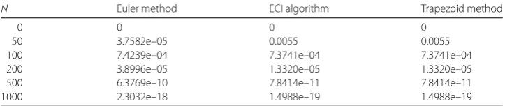
It follows from Table2and Figs.1–2that the accuracy of the numerical solutions ob-tained by the ECI algorithm is much higher than that obob-tained by Euler method, and the error approaches zero much faster. Meanwhile, Fig.3shows that this algorithm is stable for different initial values. All these facts verify the theoretical results.
Table 1 Comparison of numerical solutions for different number of steps,N, obtained by different methods
N Euler method ECI algorithm Trapezoid method
0 1.0 1.0 1.0
50 0.1353 0.1408 0.1408
100 0.0176 0.0191 0.0191
200 2.9647e–04 3.4878e–04 3.4878e–04
500 1.4235e–09 2.1396e–09 2.1396e–09
1000 1.9452e–18 4.3982e–18 4.3982e–18
Table 2 Comparison of errors for different number of steps,N, obtained by different methods
N Euler method ECI algorithm Trapezoid method
0 0 0 0
50 3.7582e–05 0.0055 0.0055
100 7.4239e–04 7.3741e–04 7.3741e–04
200 3.8996e–05 1.3320e–05 1.3320e–05
500 6.3769e–10 7.8414e–11 7.8414e–11
Figure 1Comparison of the numerical solutions in the time interval [0, 2] for two methods
Figure 2Comparison of the numerical solutions in the time interval [1, 2] for two methods
4.2 Applications in numerical simulations
We consider a nonlinear ordinary differential equation with initial value
⎧ ⎨ ⎩
dY
dt = –2Y– 2t,
Y(0) = 1.0,Y∈R.
Firstly, we make a transformation as follows. LetZ=Y+t, then we have
dZ dt =
dY dt + 1.
So dZdt = –2Z+ 1. And if we letX=Z–12, thendXdt = –2X. Therefore, the analytic solution is
Y=1 2e
–2t–t+1 2.
Secondly, the ECI algorithm is applied to this equation and the numerical solution is obtained as follows:
U(t) = 1 + 0.5a(t–nh) 1 – 0.5a(t–nh)
Yn+tn– 1 2
, nh≤t≤(n+ 1)h,a= –2,n= 0, 1, . . .
We choose the step sizeh= 0.01 and iterative stepN= 600. The numerical results are shown as the following Figs.4and5.
And we obtain the computational time when the error tolerance is no more thanE= 4.91e–06. The results are as follows.
Figures4–5and Table3demonstrate that the accuracy of the ECI algorithm is much higher than that of the trapezoid method, and the iteration times decrease obviously, so that the computational efficacy of the ECI algorithm is better than that of Euler and trape-zoid methods. Altogether, the ECI algorithm is an excellent and appropriate method for some nonlinear ODEs.
Figure 5Comparison of errors from Euler scheme and ECI algorithm
Table 3 Comparison of various characteristics for different methods
Main properties Euler method ECI algorithm Trapezoid method
computational time 4.431 3.852 4.231
number of iterations 890 773 1369
average iteration times 2.011 2.008 3.237
used CPU time 0.527 0.471 0.508
Remark3 As we see from this numerical experiment, although the ECI algorithm is con-structed for simple test equations, it can be extended to some nonlinear ODEs, which can generate dynamical systems by some parameter transformations. However, the con-ditions, which should be satisfied for such nonlinear ODEs, are still to be investigated, and the associated algorithm will be revised, if needed. All these questions will be tackled in our future work.
5 Conclusion
The main result of this paper is the dynamical analysis of the ECI algorithm and its ap-plications in simulating the solutions of ODEs. The results show that this algorithm is effective and the numerical results can match the results of theoretical analysis. Although some progress is made, more practical models and methods, which are needed to solve a system of ODEs or stochastic differential equations, will be shown in our future work.
Acknowledgements
The authors would like to express their gratitude to the referees for giving strong and very useful suggestions for improving the article.
Funding
This work is supported by the Science Research Projection of the Education Department of Fujian Province, No. JT180122, the Natural Science Foundation of Fujian Province, No. 2015J01019, and NSFC(Nos. 11021101, 11290142, 91130003, 11771149 and 11701086).
Availability of data and materials
Not applicable.
Competing interests
Authors’ contributions
All authors participated in drafting and checking the manuscript, read and approved the final manuscript.
Author details
1College of Computer and Information Science, Fujian Agriculture and Forestry University, Fuzhou, P.R. China. 2Department of Sciences and Education, Fujian Center for Disease Control and Prevention, Fuzhou, P.R. China.3Ningde
Normal University, Ningde, P.R. China.
Publisher’s Note
Springer Nature remains neutral with regard to jurisdictional claims in published maps and institutional affiliations.
Received: 17 July 2018 Accepted: 2 December 2018 References
1. Butcher, J.C.: The Numerical Analysis of Ordinary Differential Equations: Runge–Kutta and General Linear Methods. Wiley, New York (1987)
2. Haier, E.: Energy-preserving variant of collocation methods. J. Numer. Anal. Ind. Appl. Math.5, 73–84 (2010) 3. Khasminskii, R.: Stochastic Stability of Differential Equations, 2nd edn. Springer, Berlin (2011)
4. Milstein, G.: Numerical Integration of Stochastic Differential Equations. Kluwer Academic, Dordrecht (1995) 5. Wang, P.: A-stable Runge–Kutta methods for stiff stochastic differential equations with multiplicative noise. Comput.
Appl. Math.34(2), 773–792 (2015)
6. Wang, T.: Optimal point-wise error estimate of a compact difference scheme for the coupled Gross–Pitaevskii equations in one dimension. J. Sci. Comput.59, 158–186 (2014)
7. Xie, X., Chen, F.: Uniqueness of limit cycle and quality of infinite critical point of a class of cubic system. Ann. Differ. Equ.21, 3 (2005)
8. Xie, X., Zhan, Q.: Uniqueness of limit cycles for a class of cubic system with an invariant straight line. Nonlinear Anal. TMA70(12), 4217–4225 (2009)
9. Yang, Q.: Numerical Analysis, 2nd edn. Tsinghua University Press (2008)
10. Zhan, Q.: Mean-square numerical approximations to random periodic solutions of stochastic differential equations. Adv. Differ. Equ.2015, 292, 1–17 (2015)
11. Zhan, Q.: Shadowing orbits of stochastic differential equations. J. Nonlinear Sci. Appl.9, 2006–2018 (2016)
![Figure 1 Comparison of the numerical solutions in the time interval [0,2] for two methods](https://thumb-us.123doks.com/thumbv2/123dok_us/940202.1114491/7.595.118.480.539.720/figure-comparison-numerical-solutions-time-interval-methods.webp)


