Dynamical analysis in exponential RED algorithm with communication delay

R E S E A R C H

Open Access

Dynamical analysis in exponential RED

algorithm with communication delay

Changjin Xu

_{and Peiluan Li}

*_{Correspondence: [email protected]} 1_{Guizhou Key Laboratory of}

Economics System Simulation, Guizhou University of Finance and Economics, Guiyang, 550004, P.R. China

Full list of author information is available at the end of the article

Abstract

In this paper, an exponential RED algorithm with communication delay is considered. By choosing the delay as a bifurcation parameter, we demonstrate that a Hopf bifurcation would occur when the delay exceeds a critical value. Some explicit formulas are worked out for determining the stability and the direction of the bifurcated periodic solutions by using the normal form theory and center manifold theory. Finally, numerical simulations supporting the theoretical analysis are provided.

Keywords: exponential RED; stability; Hopf bifurcation; congestion control; periodic solution

1 Introduction

It is well known that Internet applications, such as the world wide web, file transfer, Usenet news and remote login, are delivered via the Transmission Control Protocol (TCP). With a spectacular growth of Internet applications, congestion control has become a subject of intense research activity. An uncontrolled network may suffer from severe congestion, which can cause high packet loss rates and increasing delays, the upper formation ap-plication systems performance drop, and it can even break the whole system by causing congestion collapse (or Internet meltdown) []. Thus congestion control is one of the crit-ical issues for the efficient operation of the Internet. Many researchers have investigated the congestion control problems of the Internet and a lot of excellent and interesting re-sults have been obtained, for example, Raina and Heckmann [] investigated the stability properties of the congestion avoidance phase of TCP with drop tail. Guoet al.[] investi-gated the stability of an exponential RED model with heterogeneous delays. Liuet al.[] studied the bifurcation and chaotic behavior of the Transmission Control Protocol (TCP) and User Datagram Protocol (UDP) network with Random Early Detection (RED) queue management. Xuet al.[] studied the Local Hopf bifurcation and global existence of pe-riodic solutions of the following TCP system:

dx(t)

dt =x(t–τ)

M( –p(x(t–τ)))

Nx(t) –

x(t)p(x(t–τ)) M

, (.)

whereM, N are two positive constants,p(y) is an increasing non-negative continuous function in (, +∞) andτis the round-trip propagation delay for each of the TCP connec-tions. Guoet al.[] considered the stability and Hopf bifurcation of the following

tion control model with two communication delays:

numbers,p(t) is the loss probability function,τiis the round-trip delay for sourcei,cis

the link capacity,kandγ are positive gain parameter,i= , . For more related work on congestion control, see [–].

Based on [–], Guoet al.[] recently studied the following exponential RED algorithm coupled with TCP-Reno with a single source and with two sources:

⎧

parameter, and the decrease factor of the sourcei, respectively. By choosing the delay as a bifurcation parameter, Guoet al.[] obtained the necessary and sufficient conditions for the existence of Hopf bifurcation and a formula for determining the direction of the Hopf bifurcation and the stability of bifurcating periodic solutions.

Motivated by [] and considering that, when the number of sources is large, the sim-plified model can reflect the really exponential RED algorithm more closely, in this paper, we consider an exponential RED algorithm coupled with TCP-Reno with a single source and with three sources, then we have the following system:

⎧

The purpose of this paper is to discuss the stability and the properties of the Hopf bifur-cation of model (.). This paper is organized as follows. In Section , the stability of the equilibrium and the existence of a Hopf bifurcation at the equilibrium are studied. In Sec-tion , the direcSec-tion of the Hopf bifurcaSec-tion and the stability and periodic of bifurcating periodic solutions on the center manifold are determined. In Section , numerical simu-lations are carried out to illustrate the validity of the main results. Some main conclusions are drawn in Section .

2 Stability of the equilibrium and local Hopf bifurcations

wherep∗satisfies the following equation:

 –p∗

βp∗ +

 –p∗

βp∗ +

 –p∗

βp∗ =cα.

Let

y(t) =x(t) –x∗_, y(t) =x(t) –x∗_,

y(t) =x(t) –x∗_, y(t) =p(t) –p∗.

(.)

Substituting (.) into (.), we obtain the following linearized system: ⎧

⎪ ⎪ ⎪ ⎨ ⎪ ⎪ ⎪ ⎩ ˙

y(t) =ay(t) +ay(t), ˙

y(t) =by(t) +by(t), ˙

y(t) =cy(t) +cy(t),

˙

y(t) =dy(t–τ) +dy(t–τ) +dy(t–τ),

(.)

where

a= –kβp∗x∗, b= –kβp∗x∗, c= –kβp∗x∗, d=kp∗,

a= –kβ(x

∗ )

 –p∗ , b= –

kβ(x∗)

 –p∗ , c= –

kβ(x∗)

 –p∗ .

Then the associated characteristic equation of (.) is

det ⎛ ⎜ ⎜ ⎜ ⎝

λ–a   –a

 λ–b  –b

  λ–c –c

–de–λτ _–de–λτ _–de–λτ _λ

⎞ ⎟ ⎟ ⎟

⎠= . (.)

Then we obtain the following fourth degree exponential polynomial equation:

λ+mλ+mλ+mλ+nλ+nλ+ne–λτ= , (.)

where

m= –(a+b+c), m=ab+ac+bc, m= –abc,

n= –(bd+cd+ad), n=bd(a+c) +cd(a+b) +ad(b+c),

n= –(abcd+abcd+abcd).

Letλ=iω,τ=τ, and substitute this into (.), for the sake of simplicity, denoteωand

τbyω,τ, respectively, Separating the real and imaginary parts, we have

n–nω

cosωτ+nωsinωτ=mω–ω, (.)

nωcosωτ–

n–nω

Taking the square on both sides of (.) and (.) and summing them up, we obtain

n–nω+ (nω)=mω–ω+mω–mω,

i.e.,

ω+ (m– n)ω+n– mm–n_ω+m+ nn–n_ω–n_= . (.)

Letp=m– n,q=n– mm–n,u=m+ nn–n,v= –n,z=ω. Then equation

(.) becomes

z+pz+qz+uz+v= . (.)

Let

l(z) =z+pz+qz+uz+v. (.)

If the coefficientski(i= , , , ),α,βj(j= , , ) of system (.) are given, it is easy to

use computer to calculate the roots of (.). Sincelimz→∞l(z) = +∞andv< , we can

conclude that (.) has at least one positive real root.

Without loss of generality, we assume that (.) has four positive roots, denoted byz, z,z,z, respectively. Then (.) has four positive roots

ω=

√

z, ω=

√

z, ω=

√

z, ω=

√

z.

By (.) and (.) we have

τ_k(j)=  ωk

arccos(mω



k–m)(n–nωk) + (mωk–mω)nω

(n–nω_k)_{+ (nω)} + jπ

, (.)

where k= , , ,  andj= , , , . . . . Then±iωk are a pair of purely imaginary roots of

equation (.) withτ=τ_k(j). Obviously, the sequence{τ_k(j)}+∞_j= is increasing, and

lim

j→+∞τ (j)

k = +∞, k= , , , .

Then we can define

τ=τk() =_≤min k≤

τ_k(), ω=ωk. (.)

Note that, whenτ= , (.) becomes

λ+qλ+qλ+qλ+q= , (.)

where

q= –(a+b+c),

q=bd(a+c) +cd(a+b) +ad(c+d) –abc,

q=abcd+abcd+abcd.

A set of necessary and sufficient conditions for all roots of (.) to have a negative real part is given by the well-known Routh-Hurwitz criteria in the following form:

q> , qq–q> , qqq–q_–q_q> , q> . (.)

Letλ(τ) =α(τ) +iω(τ) be the root of equation (.) nearτ =τ_k(j) satisfyingα(τ_k(j)) = , ω(τ_k(j)) =ωk. Then the following lemma holds.

Lemma . Suppose that l(zk)= ,where l(z)is defined by(.).Ifτ=τk(j),then±iωkare a pair of simple purely imaginary roots of equation(.).Moreover,

d(Reλ(τ))

dτ

τ=τ_k(j)

= 

and the sign of[d(Re_dλ(τ_τ ))]_τ

=τ_k(j)is consistent with that of l _(z

k).

Proof Let

F(λ) =λ+mλ+mλ+mλ, H(λ) =nλ+nλ+n. (.)

Then (.) can be written as

F(λ) +H(λ)e–λτ= , (.)

which leads to

F(λ)F(λ) –H(λ)H(λ) = . (.)

Thus, together with (.) and (.), we get

lω=F(iω)F(iω) –H(iω)H(iω). (.)

Differentiating both sides of equation (.) with respect toω, we obtain

ωlω=iF(iω)F(iω) –F(iω)F(iω) –H(iω)H(iω) +H(iω)H(iω). (.)

Ifiωkis not simple, thenωkmust satisfy

d dλ

F(λ) +H(λ)e–λτk(j)

λ=iωk

= ,

i.e.,

F(iωk) +H(iωk)e–ωkτ

(j)

k _–τ(j)

k H(iωk)e–ωkτ

(j)

By (.), we obtain

Taking the derivative ofλwith respect toτin (.), it is easy to obtain

It follows from this together with (.) that

d(Reλ(τ))

k). This completes the

proof.

Lemma .[] For the transcendental equation

Pλ,e–λτ_{, . . . ,e}–λτm_=λn_+p()

 λn–+· · ·+p () n–λ+p()n

+p()_ λn–+· · ·+p_n()_–λ+p()_ne–λτ₊· · ·

+p(_m)λn–+· · ·+p_n(m_–)λ+p(_nm)e–λτm_{= ,}

as(τ,τ,τ, . . . ,τm)vary,the sum of orders of the zeros of P(λ,e–λτ, . . . ,e–λτm)in the open right half plane can change,and only a zero appears on or crosses the imaginary axis.

From Lemma ., it is easy to obtain the following results.

Theorem . Letτ_k(j)andτbe defined by(.)and(.),respectively.

(i) If(.)holds,the equilibriumE∗(x∗_,x∗_,x∗_,p∗)of system(.)is asymptotically stable forτ∈[,τ).

(ii) If(.)andl(zk)hold,then system(.)undergoes a Hopf bifurcation at the

equilibriumE∗(x∗,x∗,x∗,p∗)whenτ=τ (j)

k ,i.e.,system(.)has a branch of periodic

solutions bifurcating from the equilibriumE∗(x∗_,x∗_,x_∗,p∗)nearτ=τ_k(j).

3 Direction and stability of the Hopf bifurcation

In the previous section, we have obtained conditions for Hopf bifurcation to occur when τ =τ_k(j). In this section, we shall derive the explicit formulas for determining the direc-tion, stability, and period of these periodic solutions bifurcating from the equilibrium

E∗(x∗,x∗,x∗,p∗) at these critical value ofτ, by using techniques from the normal form and

center manifold theory [], Throughout this section, we always assume that system (.) undergoes Hopf bifurcation at the equilibriumE∗(x∗,x∗,x∗,p∗) forτ =τ

(j)

k , and then±iωk

are corresponding purely imaginary roots of the characteristic equation at the equilibrium

E∗(x∗,x∗,x∗,p∗). The linear part of system (.) atE∗(x∗,x∗,x∗,p∗) is given by

⎧ ⎪ ⎪ ⎪ ⎨ ⎪ ⎪ ⎪ ⎩ ˙

y(t) =ay(t) +ay(t), ˙

y(t) =by(t) +by(t), ˙

y(t) =cy(t) +cy(t),

˙

y(t) =dy(t–τ) +dy(t–τ) +dy(t–τ),

(.)

and the non-linear part is given by

f(μ,ut) = (f,f,f,f)T, (.)

where

f=ay_(t) +ay(t)y(t–τ) +ay(t)y(t) +ay(t–τ)y(t)

+ay_(t) +ay_(t)y(t–τ) +ay_(t)y(t) +ay(t)y(t–τ)y(t) + h.o.t.,

f=by(t) +by(t)y(t–τ) +by(t)y(t) +by(t–τ)y(t)

+by_(t) +by_(t)y(t–τ) +by_(t)y(t) +by(t)y(t–τ)y(t) + h.o.t.,

+cy_(t) +cy_(t)y(t–τ) +cy_(t)y(t) +cy(t)y(t–τ)y(t) + h.o.t.,

f=dy(t–τ)y(t) +dy(t–τ)y(t) +dy(t–τ)y(t),

where

a=kβp∗x∗_, a= –kβp∗, a=kβx

∗

(p∗– )

 –p∗ , a=

kβx∗

 –p∗,

a= –kβp

∗

x∗_ , a= kβp∗

x∗_ , a= – kβp∗

 –p∗, a=

kβ(p∗– )

 –p∗ ,

b=kβp∗x∗, b= –kβp∗, b=

kβx∗_(p∗– )  –p∗ ,

b=kβx

∗ 

 –p∗ , b= – kβp∗

x∗_ , b= kβp∗

x∗_ ,

b= – kβp∗

 –p∗ , b=

kβ(p∗– )

 –p∗ , d=k.

Setτ=τ_k(j)+μand denote

Ck[–τ, ] =ϕ|ϕ: [–τ, ]→R, each component ofϕ

haskth order continuous derivative.

For convenience, denoteC[–τ, ] byC_{[–τ, ].}

Forϕ(θ) = (ϕ(θ),ϕ(θ),ϕ(θ),ϕ(θ))T∈C([–τ, ],R), define a family of operators

Lμϕ=Bϕ() +Bϕ(–τ) (.)

and

G(μ,ϕ) = (k,k,k,k)T_{, (.)}

where

B= ⎛ ⎜ ⎜ ⎜ ⎝

a   a

 b  b

  c c

   

⎞ ⎟ ⎟ ⎟

⎠, B=

⎛ ⎜ ⎜ ⎜ ⎝

   

   

   

d d d  ⎞ ⎟ ⎟ ⎟ ⎠,

k=aϕ_() +aϕ()ϕ(–τ) +aϕ()ϕ() +aϕ(–τ)ϕ()

+aϕ_() +aϕ_()ϕ(–τ) +aϕ(t)ϕ() +aϕ(t)ϕ(–τ)ϕ() +o

ϕ,

k=bϕ_() +bϕ()ϕ(–τ) +bϕ()ϕ() +bϕ(–τ)y()

+bϕ_() +bϕ_()ϕ(–τ) +bϕ()ϕ() +bϕ()ϕ(–τ)ϕ() +o

ϕ,

k=cϕ_() +cϕ()ϕ(–τ) +cϕ()ϕ() +cϕ(t–τ)ϕ()

+cϕ_() +cϕ_()ϕ

 –τ_k(j)+cϕ_()ϕ() +cϕ()ϕ(–τ)ϕ() +o

ϕ,

andLμis a one-parameter family of bounded linear operators inC([–τ, ],R_)→R_{. By}

the Riesz representation theorem, there exists a matrix whose components are bounded variation functionsη(θ,μ) in [–τ, ]→R_{, such that}

Lμϕ=



–τ

dη(θ,μ)ϕ(θ). (.)

In fact, choosing

η(θ,μ) =Bδ(θ) +Bδ(θ+τ), (.)

whereδ(θ) is the Dirac delta function, then (.) is satisfied. For (ϕ,ϕ,ϕ,ϕ)∈(C[–τ, ], R_{), define}

A(μ)ϕ= _dϕ(θ)

dθ , –τ≤θ< ,



–τdη(s,μ)ϕ(s), θ= 

(.)

and

Rϕ=

, –τ≤θ< ,

f(μ,ϕ), θ= . (.)

Then (.) is equivalent to the abstract differential equation

˙

ut=A(μ)ut+R(μ)ut, (.)

whereu= (u,u,u,u)T_,u

t(θ) =u(t+θ),θ∈[–τ, ].

Forψ∈C([–τ, ], (R₎∗_{), define}

A∗ψ(s) =

–dψ(_dss), s∈(,τ], 

–τdηT(t, )ψ(–t), s= .

(.)

Forφ∈C([–τ, ],R) andψ∈C([,τ], (R)∗), define the bilinear form

ψ,φ=ψ¯()φ() –



–τ

θ

ξ=

ψT(ξ–θ)dη(θ)φ(ξ)dξ, (.)

whereη(θ) =η(θ, ). We have the following result on the relation between the operators

A=A() andA∗.

Lemma . A=A()and A∗are adjoint operators.

Proof Letφ∈C_{([–τ, ],R}_{) andψ∈C}_([,τ],R₎∗_{. It follows from (.) and the}

defini-tions ofA=A() andA∗that

ψ(s),A()φ(θ)=ψ¯()A()φ() –



–τ_k(j)

θ

ξ=

¯

ψ(ξ–θ)dη(θ)A()φ(ξ)dξ

=ψ¯()



–τ_k(j)

dη(θ)φ(θ) –



–τ_k(j)

θ

ξ=

¯

=ψ¯()

This shows thatA=A() andA∗are adjoint operators and the proof is complete.

By the discussions in Section , we know that±iωkare eigenvalues ofA(), and they are

also eigenvalues ofA∗corresponding toiωkand –iωk, respectively. We have the following

result.

Lemma . The vector

q(θ) = (,r,r,r)T_eiωkθ_{, θ}∈_{[–τ, ],}

is the eigenvector of A()corresponding to the eigenvalue iωk,and

That is,

Therefore, we can easily obtain

r=

On the other hand,



Therefore, we can easily obtain

Next, we use the same notations as those in Hassardet al.[], and we first compute the coordinates to describe the center manifoldCatμ= . Letytbe the solution of equation

(.) whenμ= . Define

z(t) =q∗,yt

, W(t,θ) =yt(θ) – Re

z(t)q(θ) (.)

on the center manifoldC, and we have

W(t,θ) =Wz(t),z¯(t),θ, (.)

where

Wz(t),z¯(t),θ=W(z,z¯) =Wz 

 +Wzz¯+W ¯

z

 +· · · (.)

andzandz¯are local coordinates for center manifoldCin the direction ofq∗ andq¯∗.

Noting thatWis also real ifytis real, we consider only real solutions. For solutionsyt∈C

of (.),

˙

z(t) = q∗(s),x˙t

=q∗(s),A()ut+R()ut

= q∗(s),A()yt

+q∗(s),R()yt

= A∗q∗(s),yt

+q¯∗()R()yt

–



–τ_k(j)

θ

ξ=

¯

q∗(ξ–θ)dη(θ)A()R()yt(ξ)dξ

= iωkq∗(s),yt

+q¯∗()f,yt(θ)

def

= iωkz(t) +q¯∗()f

z(t),z¯(t). (.)

That is,

˙

z(t) =iωkz+g(z,z¯), (.)

where

g(z,z¯) =gz 

 +gz¯z+g ¯

z

 +g

zz¯

 +· · ·. (.)

Hence, we have

g(z,z¯) =q¯∗()f(z,z¯) =f(,yt)

=D¯,¯r_∗,r¯∗_,¯r_∗f(,yt),f(,yt),f(,yt),f(,yt)

T

, (.)

where

f(,yt) =ayt() +ayt()yt

–τ_k(j)+ayt()yt() +ayt

–τ_k(j)yt()

+ay_t() +ay_t()yt

+r_∗

unknown ing, we still need to compute them. From (.), (.), we have

Comparing the coefficients, we obtain

(A– iω)W(θ) = –H(θ), (.)

AW(θ) = –H(θ), (.)

. . . .

And we know that forθ∈[–τ_k(j), ),

Comparing the coefficients of (.) with (.) gives

H(θ) = –gq(θ) –g¯ q¯(θ), (.)

H(θ) = –gq(θ) –g¯ q¯(θ). (.)

From (.), (.), and the definition ofA, we get

˙

W(θ) = iωkW(θ) +gq(θ) +g¯q¯(θ). (.)

Noting thatq(θ) =q()eiωθ_{, we have}

W(θ) =ig ωk

q()eiωkθ₊ig¯

ωk¯

q()e–iωkθ_+Eeiωkθ_{, (.)}

whereE is a constant vector. Similarly, from (.), (.), and the definition ofA, we have

˙

W(θ) =gq(θ) +g¯ q¯(θ), (.)

W(θ) = –ig ωk

q()eiωkθ₊ig¯

ωk ¯

q()e–iωkθ_{+E, (.)}

whereEis a constant vector.

In the following, we shall seek appropriateE,Ein (.), (.), respectively. It follows

from the definition ofAand (.), (.) that



–τ_k(j)

dη(θ)W(θ) = iωkW() –H() (.)

and



–τ_k(j)

dη(θ)W(θ) = –H(), (.)

whereη(θ) =η(,θ). From (.), we have

H() = –gq() –g¯ q¯() + (H,H,H,H)T, (.)

where

H= 

a+ae–iωkτ

(j)

k +a_r_+a_r_e–iωkτ

(j)

k ,

H= 

br+bre–iωkτ

(j)

k +b_r_r_+b_r_r_e–iωkτk(j),

H= 

cr+cre–iωkτ

(j)

k +c_r_r_+c_r_r_e–iωkτk(j),

H= 

dre–iωkτ

(j)

From (.), we have

=det

Similarly, substituting (.) and (.) into (.), we have

(a) (b)

(c) (d)

Figure 1 Dynamic behavior of system (4.1): times series ofxi(i= 1, 2, 3) andp(t).A Matlab simulation of the asymptotically stable origin to system (4.1) withτ= 1.65 <τ0≈1.85. The initial value is (0.5, 0.5, 0.5, 0.5).

=det

⎛ ⎜ ⎜ ⎜ ⎝

a –P  a

 –P  b

 –P c c

d –P d  ⎞ ⎟ ⎟ ⎟ ⎠,

=det

⎛ ⎜ ⎜ ⎜ ⎝

a  –P a

 b –P b

  –P c

d d –P 

⎞ ⎟ ⎟ ⎟ ⎠,

=det

⎛ ⎜ ⎜ ⎜ ⎝

a   –P

 b  –P

  c –P d d d –P

⎞ ⎟ ⎟ ⎟ ⎠.

From (.), (.), (.), (.), we can calculategand derive the following values:

c() = i ωk

!

gg– |g|–|g|



 "

+g  ,

μ= –

(a) (b)

(c) (d)

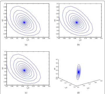
Figure 2 Dynamic behavior of system (4.1): projection onx1-p,x2-p,x3-pplane and projection on

x2-x3-pspace.A Matlab simulation of the asymptotically stable origin to system (4.1) with

τ= 1.65 <τ0≈1.85. The initial value is (0.5, 0.5, 0.5, 0.5).

β= Re

c(),

T= –Im{c()}+μIm{λ

_(τ(j) k )}

ωk

.

These formulas give a description of the Hopf bifurcation periodic solutions of (.) at τ =τ_k(j) on the center manifold. From the discussion above, we have the following re-sult.

Theorem . For system(.),if(H)-(H)hold,the periodic solution is supercritical( sub-critical)ifμ>  (μ< );the bifurcating periodic solutions are orbitally asymptotically stable with asymptotical phase(unstable)ifβ<  (β> );the periods of the bifurcating periodic solutions increase(decrease)if T>  (T< ).

4 Numerical examples

(a) (b)

(c) (d)

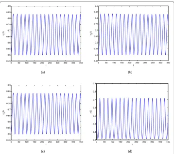
Figure 3 Dynamic behavior of system (4.1): times series ofxi(i= 1, 2, 3) andp.A Matlab simulation of a periodic solution to system (4.1) withτ= 1.97 >τ0≈1.85. The initial value is (0.5, 0.5, 0.5, 0.5).

consider the following special case of system (.):

⎧ ⎪ ⎪ ⎪ ⎪ ⎨ ⎪ ⎪ ⎪ ⎪ ⎩ ˙

x(t) = .x(t–τ)[_.–p_x(t)

(t)– .x(t)p(t)],

˙

x(t) = .x(t–τ)[_.–p_x(t)

(t)– .x(t)p(t)],

˙

x(t) = .x(t–τ)[_.–p_x(t)

(t)– .x(t)p(t)],

˙

p(t) = .p(t)[x(t–τ) +x(t–τ) +x(t–τ) – ].

(.)

By some complicated computation by means of Matlab ., we getω≈.,τ≈.,

λ(τ)≈. – .i. Thus we can calculate the following values:c()≈–. –

.i, μ≈., β≈–.,T≈.. We see that the conditions

indi-cated in Theorem . are satisfied. Furthermore, it follows thatμ>  andβ< . Choose

τ = . <τ≈.. Thus, the equilibrium (x∗,x∗,x∗,p∗) is stable when τ <τ, which

is illustrated by the computer simulations (see Figure  and Figure ). When τ passes through the critical value τ≈., the equilibrium (x∗,x∗,x∗,p∗) loses its stability and

a Hopf bifurcation occurs,i.e., a family of periodic solutions bifurcate from the equilib-rium (x∗_,x∗_,x∗_,p∗). Chooseτ= . >τ≈.. Sinceμ>  andβ< , the direction of

the Hopf bifurcation isτ >τ, and these bifurcating periodic solutions from (x∗,x∗,x∗,p∗)

(a) (b)

(c) (d)

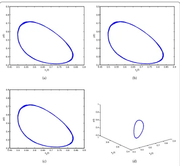
Figure 4 Dynamic behavior of system (4.1): projection on thex1-p,x2-p,x3-pplane and projection on

thex2-x3-pspace, respectively.A Matlab simulation of a periodic solution to system (4.1) with

τ= 1.97 >τ0≈1.85. The initial value is (0.5, 0.5, 0.5, 0.5).

5 Conclusions

In this paper, we have investigated the properties of Hopf bifurcation in an exponen-tial RED algorithm with communication delay. It is shown that under certain conditions, the Hopf bifurcation occurs as the delayτ passes through some critical valuesτ =τ_k(j),

k,j= , , , . . . . Moreover, the direction of the Hopf bifurcation and the stability of the bi-furcating periodic orbits are derived by applying the normal form theory and the center manifold theorem.

Competing interests

The authors declare that they have no competing interests.

Authors’ contributions

The authors have made contributions of the same significance. All authors read and approved the final manuscript.

Author details

1_{Guizhou Key Laboratory of Economics System Simulation, Guizhou University of Finance and Economics, Guiyang,}

550004, P.R. China.2_{School of Mathematics and Statistics, Henan University of Science and Technology, Luoyang, 471023,} P.R. China.

Acknowledgements

Science Foundation of China (No. 11101126). The authors would like to thank the referees and the editor for helpful suggestions incorporated into this paper.

Received: 10 October 2015 Accepted: 28 November 2015

References

1. Liu, F, Guan, ZH, Wang, HO: Controlling bifurcations and chaos in TCP-UDP-RED. Nonlinear Anal., Real World Appl.

11(3), 1491-1501 (2010)

2. Raina, G, Heckmann, O: TCP: local stability and Hopf bifurcation. Perform. Eval.64, 266-275 (2007)

3. Guo, ST, Liao, XF, Li, CD, Yang, DG: Stability analysis of a novel exponential-RED model with heterogeneous delays. Comput. Commun.30, 1058-1074 (2007)

4. Xu, CJ, Tang, XH, Liao, MX: Local Hopf bifurcation and global existence of periodic solutions in TCP system. Appl. Math. Mech.31(6), 775-786 (2010)

5. Guo, ST, Feng, G, Liao, XF, Liu, Q: Novel delay-range-dependent stability analysis of the second-order congestion control algorithm with heterogenous communication delays. J. Netw. Comput. Appl.32, 568-577 (2009) 6. Tian, YP: A general stability criterion for congestion control with diverse communication delays. Automatica41,

1255-1262 (2005)

7. Abdallah, CT, Chiasson, J, Tarbouriech, S (eds.): Advances in Communication Control Networks. Lecture Notes in Control and Information Sciences. Springer, Berlin (2004)

8. Srikant, R: The Mathematics of Internet Congestion Control. Birkhäuser, Boston (2004)

9. Liu, S, Basar, T, Srikant, R: Exponential-RED: a stabilizing AQM scheme for low-and high-speed TCP protocols. IEEE/ACM Trans. Netw.13(5), 1068-1081 (2005)

10. Alpcan, T, Basar, T: A globally stable adaptive congestion control scheme for Internet-style networks with delays. IEEE/ACM Trans. Netw.13(6), 1261-1274 (2005)

11. Raina, G: Local bifurcation analysis of some dual congestion control algorithms. IEEE Trans. Autom. Control50(8), 1135-1146 (2005)

12. Sichitiu, ML, Bauter, PH: Asymptotic stability of congestion control systems with multiple sources. IEEE Trans. Autom. Control51(2), 292-298 (2006)

13. Guo, ST, Liao, XF, Liu, Q, Li, CD: Necessary and sufficient conditions for Hopf bifurcation in exponential RED algorithm with communication delay. Nonlinear Anal., Real World Appl.9(4), 1768-1793 (2008)

14. Ruan, S, Wei, J: On the zero of some transcendental functions with applications to stability of delay differential equations with two delays. Dyn. Contin. Discrete Impuls. Syst., Ser. A Math. Anal.10, 863-874 (2003)