Brain Tumor Detection Using Neural Network
Vaishnavi S. Mehekare1, Dr.S.R.Ganorkar2,
Department of Electronics & Telecommunication, Sinhgad College of Engineering, Savitribai Phule Pune University, Pune, India.
ABSTRACT: Among cerebrum tumors, Glioma are the most widely recognized, forceful, prompting a short future in their most elevated evaluation. Thus, treatment arranging is a key stage to move forward the personal satisfaction of oncological patients. Thus, programmed and reliable techniques are required. Propose a automatic division strategy in light of Convolutional Neural Networks (CNN), investigating little 33 kernel. The use of this kernel permits outlining a more profound design, other than having a constructive outcome against over fitting, given the less number of weights in the system. We also examined the utilization of power standardization as a pre-preparing step, which however not basic in CNN-based division techniques, ended up being exceptionally powerful for mind tumor division in MRIpictures.
KEYWORDS: MRI, Feature Extraction, Segmentation, Gabor, BPN
I. INTRODUCTION
Glioma is a broad category of brain and spinal cord tumors that come from glial cells, brain cells that can develop into tumors. Low-grade versions of gliomas can occur in children. Brain tumors are slightly more likely to occur in males. Prior radiation to the brain is a risk factor for malignant gliomas. The precise Segmentation of gliomas and its intra-tumoral structures is imperative for treatment arranging, as well as for follow-up assessments [1]. Be that as it may, it is a testing assignment, since the shape, structure, and area of these anomalies are profoundly factor. In mind tumor division, we discover a few techniques that expressly build up a parametric or non-parametric probabilistic model for the basic information. Automatic and reliable segmentation methods are required; however, the large spatial and structural variability among brain tumors make automatic segmentation a challenging problem. In this paper, we propose an automatic segmentation method based on Convolutional Neural Networks (CNN), exploring small 3×3 kernels. We also investigated the use of intensity normalization as a pre-processing step, which though not common in CNN-based segmentation methods, proved together with data augmentation to be very effective for brain tumorsegmentation.
II. MOTIVATION
Glioma leads to very short life expectancy. In previous techniques of segmentation the accuracy of the algorithms is less. Making use of an automatic segmentation method based on Convolutional Neural Networks (CNN) to overcome above drawbacks. The symptoms, prognosis, and treatment of a malignant glioma depend on the person’s age, the exact type of tumor, and the location of the tumor within the brain. Previously many techniques are applied to detect the brain tumor segmentation and detection[6]. Magnetic resonance imaging (MRI) is a noninvasive method for producing three-dimensional (3D) tomographic images of the human body. MRI is most often used for the detection of tumors, lesions, and other abnormalities in soft tissues, such as the brain. Clinically, radiologists qualitatively analyze films produced by MRIscanners.
III. LITERATURE REVIEW
information [1]. The accurate segmentation of gliomas and its intra-tumoral structures is important not only for treatment planning, but also for follow-up evaluations.
For these reasons, accurate semi automatic or automatic methods are required [1],[6].However, it is a challenging task, since the shape, structure, and location of these abnormalities are highly variable. Additionally, the tumor mass effect changes the arrangement of the surrounding normal tissues [6]. Other methods known as Deep Learning deal with representation learning by automatically learning an hierarchy of increasingly complex features directly from data [2]. So, the focus is on designing architectures instead of developing handcrafted features, which may require specialized knowledge [18]. CNNs have been used to win several object recognition [19], [20] and biological image segmentation [21] challenges.
Since a CNN operates over patches using kernels, it has the advantages of taking context into account and being used with raw data. In the field of brain tumor segmentation, recent proposals also investigate the use of CNNs [21] – [27]. Zikic et al. [21] used a shallow CNN with two convolutional layers separated by max-pooling with stride 3, followed by one fully-connected (FC) layer and a softmax layer. Urban et al. [22] evaluated the use of 3D filters, although the majority of authors opted for 2D filters [22]–[27]. 3D filters can take advantage of the 3D nature of the images, but it increases the computational load. The large spatial and structural variability in brain tumors are also an important concern that we study using dataaugmentation.
IV. PROPOSED SYSTEM
The figure below shows the existing system of the detection of brain tumor segmentation. In this method, the pre- processing is used to enhancement of the image without altering the information content. The main causes of image imperfections are as Low resolution, Simulation, Presence of image artifacts, Geometric Distortion, Low contrast, High level of noise. The feature Extraction is used to extract the feature from the image. This system gives the moderate result i.e. the detection of the tumor is accurate but the classification of the tumor is not done in the circuit.
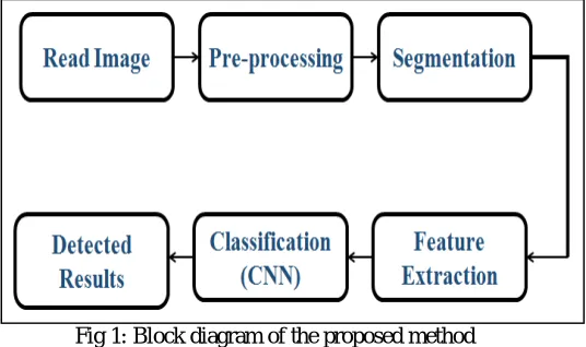
Fig 1: Block diagram of the proposed method
There are different stages: pre-processing, segmentation, feature extraction & classification using Convolutional neural network. The brief description of each step of the block diagram is given below.
A. Pre-Processing:
Pre-Processing strategies point the upgrade of the picture without changing the data content. The primary driver of picture flaws are as Low determination, Simulation, Presence of picture antiquities, Geometric Distortion, Low complexity, High level of clamor. The most applicable and essential pre-preparing systems for MRI pictures before managing cerebrum tumors is division.
Ci(k) =[(x,y):(g(x,y)-f(x,y,a,m))2 < Ɛ and (x,y) is a4-neighbor of R (k)
i i
(k)
i i i i i
B. Segmentation:
Locale developing is a basic district based picture division strategy. It is additionally delegated a pixel-based picture division strategy since it includes the determination of introductory seed focuses. This way to deal with division inspects neighboring pixels of introductory seed focuses and figures out if the pixel neighbors ought to be added to the district. The procedure is iterated on, in an indistinguishable way from general information grouping calculations. A general discourse of the locale developing calculation is depicted underneath.
1.Parcel the picture into starting seed districts R(0) .(0)(0)
2.Fit the planar model to each seed district. In the event that E(Ri
its model; otherwise dismiss it.,a,m) is sufficiently little, acknowledge RiandFor every district, find all focuses that are
perfect with the area by considering the neighbors of thelocale.
(1)
3.In the event that there were no perfect focuses, then m= m+1. In the event that m > M, don't develop Rifurther;
generally, go to step 3.
4.From the new district R(k+1)= R(k)
UC(k) , refit the model to R(k+1)and register E(R(0),a,m) .
5.Register the distinctionblunder:
6.In the event that ρ(k) < T1, go to step3.
7.m = m + 1. On the off chance that m > M, don't develop districtfacilitate.2)
8. Refit the locale at the new model f(x,y,a,m). In the event that the blunder of fit declines, acknowledge the new model and go to step3; something else, don't develop the districtfacilitate.
(2)
9. Refit the locale at the new model f(x,y,a,m). In the event that the blunder of fit declines, acknowledge the new model and go to step3; something else, don't develop the districtfacilitate.
B. FeatureExtraction:
The next step for diagnosis is to extract features. Highlight extraction is the way toward characterizing an arrangement of components, or picture attributes, which will most effectively or seriously speak to the data that is critical for investigation and characterization. Features themselves can be classified as pixel intensity based features, calculated pixel intensity-based features, and edge and texture-based features. Normal element extraction strategies incorporate Histogram of Oriented Gradients (HOG), Speeded Up Robust Features (SURF), Local Binary Patterns (LBP), Haar wavelets, and shading histograms.
LBP (Local Binary Patterns):
The local binary pattern [7] is a simple, quick, and very efficient method for extracting feature from image texture. In this method, first a neighborhood of an image is selected. Then, the intensity of the points existing in this neighborhood is compared with the intensity of the pixel located in the center of the neighborhood and a binary code is considered for each pixel according to equation(3).
In order to make the algorithm rotation-invariant usually circular neighborhood is considered. The pixels whose coordinates are not exactly located on the neighborhood of pixel center are obtained by interpolation. In equation 3, P represents the number of neighborhood pixels of a considered center pixel, R is the neighborhood radius, ɡi is the
intensity of the neighborhood pixels, and ɡc is the intensity of the centralpixel.
Ρ(k) = E(R (k+1),a,m)- E(R (k),a,m)
C. Convolutional NeuralNetwork:
Convolutional Neural Network (CNN) issued to achieve some breakthrough results and win well-known contests. The application of Convolutional layers consists in convolving a signal or an image with kernels to obtain feature maps. So, a unit in a feature map is connected to the previous layer through the weights of the kernels. The weights of the kernels are adapted during the training phase by back propagation, in order to enhance certain characteristics of the input. CNN are easier to train and less prone to overfitting. Methodology like mentioned earlier in the report, we use a patch based segmentation approach. The Convolutional network architecture and implementation are
carried out using CAFFE. CNNs are the continuation of the multi-layer Perceptron. In the MLP, a unit performs a simple computation by taking the weighted sum of all other units that serve as input to it. The network is organized into layers of units in the previous layer. The essence of CNNs is the convolutions. The main trick with Convolutional networks that avoids the problem of too many parameters is sparse connections. Every unit is not connected to every other unit in the previous layer, like in traditional neural networks. The following concepts are important in the context of CNN[1]:
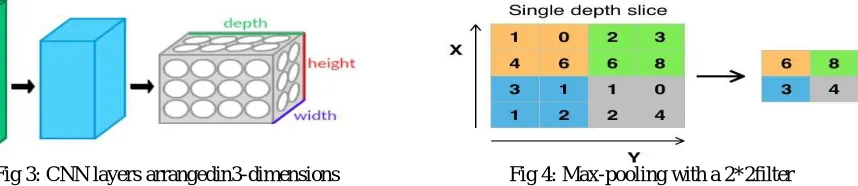
Fig 3: CNN layers arrangedin3-dimensions Fig 4: Max-pooling with a 2*2filter
a) Initialization: It is important to achieve convergence. We use the Xavier initialization. With this, the activations andthegradientsaremaintainedincontrolledlevels, otherwiseback-propagatedgradientscouldvanishorexplode.
b) Activation Function: It is responsible for non-linearly transforming the data. Rectifier linear units (ReLU), Defined as
f(x)=max(0,x), (4)
Were found to achieve better results than the more classical sigmoid, or hyperbolic tangent functions, and speed up training. However, imposing a constant 0 can impair the gradient flowing and consequent adjustment of the weights. We cope with these limitations using a variant called leaky rectifier linear unit (LReLU) that introduces a small slopeon the negative part of the function. This function is definedas
f(x) =max(0,x)+αmin(0,x) (5)
Where α is the leakyness parameter. In the last FC layer, we use softmax.
d) Regularization: It is used to reduce over-fitting. We use Drop out in the FC layers. In each training step, it removes nodes from the network with probability p. In this way, it forces all nodes of the FC layers to learn better representations of the data, preventing nodes from co-adapting to each other. At test time, all nodes are used. Dropout can be seen as an ensemble of different networks and a form of bagging, since each network is trained with a portion of the trainingdata.
e) Data Augmentation: It can be used to increase the size of training sets and reduce overfitting. Since the class of the patch is obtained by the central voxel, we restricted the data augmentation to rotating operations. Some authors also consider image translations, but for segmentation this could result in attributing a wrong class to the patch. So, we increased our data set during training by generating new patches through the rotation of the original patch. In our proposal, we used angles multiple of 90◦, although another alternative will beevaluated.
f) LossFunction:Itisthefunctiontobeminimizedduringtraining.WeusedtheCategoricalCross-entropy,
H=−∑j∈rose1s∑k∈c1assesCj,klog(Cˇj,k) (6)
Where Cˇ represents the probabilistic predictions (after the softmax) and C is the target. The high-level reasoning in the neural network is done via fully connected layers.
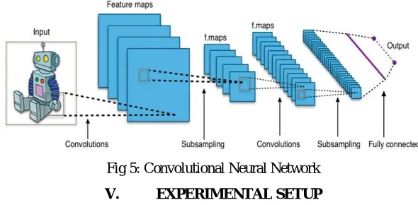
Fig 5: Convolutional Neural Network
V. EXPERIMENTAL SETUP
The MATLAB functions have been used to calculate the values of various parameters of the images. These values are to be used to differentiate whether a given MR image is normal or tumor containing. Hundred different images are used as training and testing set. Twenty-six of these images are normal MR images whereas the rest Seventy- four are images bearingtumors.
The parameters of these images are arranged into a matrix form and fed to the Convolutional neural network. We aim at a reliable segmentation method; however, brain tumors present large variability in intra-tumoral structures, which makes the segmentation a challenging problem. To reduce such complexity, we designed a CNN and tuned the intensity normalization transformation for eachtumor.
Table I: Architecture of the CNN
Layers Filter type Filter dimensions Number of filters
Layer 1 input 28*28*1 -
Layer 2 conv 9*9 20
Layer 3 pool 2*2 -
Layer 4 stack2line - -
Layer 6 sigmoid 60 -
Layer 7 softmax 10 -
In inputs, the first dimension refers to the number of channels and the next two to the size of the patch, or feature maps. Conv. refers to Convolutional layers and Max-pool. to max-pooling.
VI. RESULTS
1] Image Resizing: The images acquired after removing the header are of various sizes. In order to be able to perform matrix arithmetic’s on the images it is necessary for the images to be square matrix. Therefore all the images procured after removing the header are resized to a standard dimension of 256 × 256 pixels. The resizing of the images is done in MATLAB. The images are read using ‘imread’ and are resized using inbuilt MATLAB function ‘imresize’.
2] Image Segmentation using Region Growing Method: Image segmentation groups pixels into regions, and hence defines object regions. Common segmentation approaches to MR images are thresholding, edge detecting, clustering, genetic algorithms, and probabilistic techniques. In this work, region growing method has been used for segmentation.
3] Feature Extraction using Local Binary Pattern: In the next step, we extract features from the specific regions of tumor we found. Here, texture-based features are extracted for which local binary pattern approach is used as it gives betterrecognition.
4] Classification using Convolutional Neural Network: Convolutional neural Network is easier for training and testing purpose. It is less complex and more efficient as it avoids the problem of too many parameters. The classifier detects and locates the tumor in abnormal brain image.
ABNORMAL BRAIN IMAGE:
Fig 7: Results of abnormal brain image as input
NORMAL BRAIN IMAGE:
VII. PERFORMANCE EVALUATION
Performance of proposed method is evaluated using confusion matrix. The table shows the confusion matrix for following data.
Total Images=100 Actual Abnormal Images=74 Actual Normal Images =26
Table II : Confusion Matrix
Total Images (T) =100Predicted Normal Images Predicted Abnormal Images
Actual Normal Images (TN) = 16
Predicted as normal images, & it was actually true
(FP) = 10
Predicted as abnormal images, but they were actually normal images
Actual Abnormal Images (FN) = 4
Predicted as normal images, but they were actually abnormal
(TP) = 70
Predicted as abnormal images, & it was actually true
Table III : Parameter Analysis
Parameters Convolutional Neural network
Accuracy = (TP + TN) /T 86%
Misclassification Rate = (FP + FN) / T 14%
Precision = TN / TN + FP 61%
Sensitivity = TP / TP + FN 94%
VIII. CONCLUSION
In this paper we propose a novel CNN-based technique for division of brain tumors in MRI images. We begin by a pre-preparing stage, then feature extraction, image segmentation and post-processing. Also, various existing segmentation methods for brain MR image have been discussed. We are able to successfully implement a Convolutional Neural Network based approach to segment tumors from MRI scans using a moderately deep network with not too many parameters. We are able to get high classification accuracy.
REFERRENCES
[1] S. Bauer et al., “A survey of mri-based medical image analysis for brain tumor studies,” Physics in medicine and biology, vol. 58, no. 13, pp. 97– 129, 2013.
[2]S´ergio Pereira, Adriano Pinto, Victor Alves and Carlos A. Silva,”Brain Tumor Segmentation using Convolutional Neural Networks in MRIImages”,2016.
[3] Pavel Dvorak &BjoernMenze,”Structured Prediction with Convolutional Neural Networks for Multimodal Brain Tumor Segmentation, MICCAI-BRATS 2015.
[4] Sheela.V. K and Dr. S. Suresh Babu,”Processing Technique for Brain Tumor Detection and Segmentation,” International Research Journal of Engineering and Technology Volume: 02, June-2014
[5] Jaypatel and KaushalDoshi, “A study of Segmentation Method for detection of Tumor in Brain”, Advance in Electronic & Electric Engineering, 2014.
[6] B. Menze et al., “The multimodal brain tumor image segmentation benchmark (brats),” IEEE Transactions on Medical Imaging, vol. 34, no. 10, pp. 1993–2024, 2015.
[7]J.Selvakumar, A.Lakshami&T.Arivoli,“Brain Tumor Segmentation and Its Area Calculation using K-mean Clustering & Fuzzy C-Mean Algorithm”,IEEE-International Conference On Advances In Engineering,March30,2012.
[8] RaunaqRewari, ”Automatic Tumor Segmentation Using Convolutional Neural Network.”
[9] Stefan Bauer, Roland Wiest and Lutz-P Nolte,”A Survey Of MRI-based medical image analysis for Brain Tumor Studies”.
[11] V.Karthikeyan*1, V.J.Vijayalakshmi*2, P.Jeyakumar*3, “A Novel Approach For The Enrichment Of Digital Images Using Morphological Operators”, 2013.
[12] K.Sreedhar and B.Panlal, Enhancement of images using morphological transformation, 2012. [13] Divya Madaan1, SusheelKumar,“A New Approach for Improvement of Dark Images” , July 2012 .
[14] M. Monica Subashini*, Sarat Kumar Sahoo , “Brain Tumor Detection Using Pulse Coupled Neural Network (PCNN) and Back Propagation Network”,2012.
[15] V. SalaiSelvam and S. Shenbagadevi “Brain Tumor Detection using Scalp EEG with Modified Wavelet-ICA and Multi Layer Feed Forward Neural Network”, 2011.
[16]Y. Bengio, A. Courville, and P. Vincent, “Representation learning: A review and new perspectives,” Pattern Analysis and Machine Intelligence, IEEE Transactions on, vol. 35, no. 8, pp. 1798–1828, 2013.
[17] Y. LeCun, Y. Bengio, and G. Hinton, “Deep learning,” Nature, vol. 521, no. 7553, pp. 436–444, 2015.
[18] A. Krizhevsky, I. Sutskever, and G. E. Hinton, “Imagenet classification with deep convolutional neural networks,” in Advances in neural
information processing systems, 2012, pp. 1097–1105.
[19] S. Dieleman, K. W. Willett, and J. Dambre, “Rotation-invariant convolutional neural networks for galaxy morphology prediction,” Monthly Notices of the Royal Astronomical Society, vol. 450, no. 2, pp. 1441– 1459, 2015.
[20] D. Ciresan et al., “Deep neural networks segment neuronal membranes in electron microscopy images,” in Advances in neural information processing systems, 2012, pp. 2843–2851.
[21] D. Zikic et al., “Segmentation of brain tumor tissues with convolutional neural networks,” MICCAI Multimodal Brain Tumor Segmentation Challenge (BraTS), pp. 36–39, 2014.
[22] G. Urban et al., “Multi-modal brain tumor segmentation using deep convolutional neural networks,” MICCAI Multimodal Brain Tumor Segmentation Challenge (BraTS), pp. 1–5, 2014.
[23] A. Davy et al., “Brain tumor segmentation with deep neural networks,” MICCAI Multimodal Brain Tumor Segmentation Challenge (BraTS), pp. 31–35, 2014.
[24] M. Havaei et al., “Brain tumor segmentation with deep neural networks,” arXiv:1505.03540v1, 2015. [Online]. Available: http://arxiv.org/abs/1505.03540
[25] M. Lyksborg et al., “An ensemble of 2d convolutional neural networks for tumor segmentation,” in Image Analysis. Springer, 2015, pp. 201– 211.
[26] V. Rao, M. Sharifi, and A. Jaiswal, “Brain tumor segmentation with deep learning,” MICCAI Multimodal Brain Tumor Segmentation Challenge
(BraTS), pp. 56–59, 2015.
[27] P. Dvo˘ r´ ak and B. Menze, “Structured prediction with convolutional neural networks for multimodal brain tumor segmentation,” MICCAI