TOPSIS Based Algorithm for Solving Multi-objective Multi-level Programming Problem with Fuzzy Parameters

(1)

Article

1 TOPSIS Based Algorithm for Solving Multi-objective

2 Multi-level Programming Problem with Fuzzy

3 Parameters

4

Surapati Pramanik 1, *_{, Partha P. Dey}2_{and Florentin Smarandache}3

5

1_{Department of Mathematics, Nandalal Ghosh B.T. College, Panpur, P.O.-Narayanpur, District}_–_{North 24}

6

Parganas, Pin code-743126,West Bengal, India; e-mail: [email protected]

7

2_{Department of Mathematics, Jadavpur University, Kolkata-700032, West Bengal, India; e-mail:}

8

[email protected]

9

3_{Mathematics & Science Department, University of New Mexico, 705 Gurley Ave., Gallup, NM 87301, USA;}

10

[email protected]

11

* Correspondence: e-mail: [email protected]; Tel.: +91-9477035544

12

Abstract: The paper proposes TOPSIS method for solving multi-objective multi-level programming

13

problem (MO-MLPP) with fuzzy parameters via fuzzy goal programming (FGP). At first,λ- cut

14

method is used to transform the fuzzily described MO-MLPP into deterministic MO-MLPP. Then,

15

for specificλ, we construct the membership functions of distance functions from positive ideal

16

solution (PIS) and negative ideal solution (NIS) of all level decision makers (DMs). Thereafter, FGP

17

based multi-objective decision model is established for each level DM for obtaining individual

18

optimal solution. A possible relaxation on decisions for all DMs is taken into account for

19

satisfactory solution. Subsequently, two FGP models are developed and compromise optimal

20

solutions are found by minimizing the sum of negative deviational variables. To recognize the

21

better compromise optimal solution, the concept of distance functions is utilized. Finally, a novel

22

algorithm for MO-MLPP involving fuzzy parameters is provided and an illustrative example is

23

solved to verify the proposed procedure.

24

Keywords: multi-objective multi-level programming; fuzzy parameters; TOPSIS; fuzzy goal

25

programming; multi-objective decision making

26

27

1. Introduction

28

Multi-level programming (MLP) technique is a powerful analytical device for describing

29

decentralized planning problems involving several decision makers (DMs) in a hierarchical

30

organization. MLP has diverse practical applications in such fields as agricultural economics [1],

31

conflict resolution [2], network design [3], pollution control policies [4], warfare [5], and so on. In a

32

multi-level programming problem (MLPP), there exists a single and independent DM at each level

33

and each level DM attempts to optimize its objective function over a common feasible region but the

34

decision of each level DM is exaggerated by the actions and reactions of the other DMs.

35

Consequently, decision deadlock may occur in the decision making circumstances. However, it has

36

been observed that each level DM should have a motivation to cooperate with each other, and a

37

minimal level of satisfaction of all level DMs must be considered for overall profit of the hierarchical

38

structure.

39

Using the idea of tolerance membership function of fuzzy set theory [6] to MLPPs for

40

satisfactory decisions, Lai [7] incorporated an efficient fuzzy approach at first in 1996. Shih et al. [8]

41

(2)

and Shih and Lee [9] applied non-compensatory max-min aggregation operator and compensatory

42

fuzzy operator respectively for solving MLPPs. Sakawa et al. [10] criticized Lai et al.’s method [7]

43

and claimed that the method discussed in [7] may produce undesirable solution to the MLPPs when

44

the fuzzy goals of objective function and decision variables of upper level DM are inconsistent. In

45

order to get rid of such situations, Sakawa et al. [10] proposed an interactive fuzzy programming

46

(IFP) for MLPPs by removing the fuzzy goals of the decision variables. Sinha [11, 12] proposed fuzzy

47

mathematical programming for solving MLPPs through a supervised search procedure. Pramanik

48

and Roy [13] proposed fuzzy goal programming (FGP) models to MLPPs by taking into

49

consideration of the relaxation of decision of the upper DMs for proper allocation of decision powers

50

to the DMs within the hierarchical organization. Baky [14] presented alternative FGP models for

51

solving multi-objective MLPP (MO-MLPP) to get the highest degree of each of the membership goals

52

by minimizing over and under deviational variables.

53

In 2000, Sakawa et al. [15] presented IFP for obtaining satisfactory solution to MLPPs with fuzzy

54

parameters by updating the satisfactory degree of DMs in view of of the overall satisfactory balance

55

among all DMs. Zhang et al. [16] derived an approximation branch and bound algorithm for solving

56

decentralized multi-objective bi-level decision making with fuzzy demands. Gao et al. [17]

57

developed λ-cut and goal programming based approach for solving fuzzy linear multi-objective

58

bi-level decision problems and presented a case study on a newsborn problem. Pramanik [18]

59

formulated three novel and effective FGP models in order to solve bi-level programming problem

60

(BLPP) with fuzzy parameters by considering preference bounds of upper and lower level DMs and

61

distance function is used to select better compromise optimal solution. Pramanik [19] also

62

presentedλ- cut and FGP based models for MLPP with fuzzy parameters by extending the concept

63

discussed in [18]. Pramanik and Dey [20] solved multi-objective BLPP (MO-BLPP) involving fuzzy

64

parameters based on FGP approach due to Pramanik and Dey [21] and presented an algorithm with

65

termination criteria. Baky et al. [22] extended the concept of Pramanik and Dey [20] and proposed an

66

alternative FGP approach for solving MO-BLPP with fuzzy demands by taking into consideration of

67

the relaxation on decision of upper level DM and obtained solutions of both level DMs by

68

minimizing over and under deviational variables. Baky and Sayed [23] proposed a hybrid approach

69

of TOPSIS and FGP for MO-BLPP with fuzzy parameters. Baky and Sayed [24] studied FGP method

70

to solve MO-BLPP with fuzzy parameters using TOPSIS and modified TOPSIS techniques.

71

TOPSIS is a familiar multi-attribute decision making method which was developed by Hwang

72

and Yoon [25] is based on the principle that a DM selects an alternative which is nearest from

73

positive ideal solution (PIS) and farthest from negative ideal solution (NIS). Abo- Sinna et al. [26]

74

and Abo- Sinna and Amer [27] investigated TOPSIS for multi-objective large scale non-linear

75

programming problems with block angular structure and max-min operator is used to resolve the

76

conflict between new criteria. Abo- Sinna and Abou-El-Enien [28] presented a TOPSIS based

77

interactive algorithm for large scale multi-objective programming problem involving fuzzy

78

parameters. Baky [29] proposed two interactive TOPSIS algorithms for solving non-linear

79

MO-MLPPs. Recently, Dey et al. [30] investigated TOPSIS scheme for linear fractional MO-BLPP

80

through FGP approach by assigning preference bounds on the decision variables to reach the

81

optimal solution.

82

In this paper, we have extended the concept of Dey et al. [25] for solving MO-MLPP with fuzzy

83

parameters using FGP procedure. The remainder of the paper is structured in the following way.

84

(3)

formulation of MO-MLPP with fuzzy parameters is exhibited. Section 4 provides deterministic

86

formulation of MO-MLPP with fuzzy parameters usingλ- cut technique. Some basic concepts

87

relating to distance measures are briefly stated in section 5.TOPSIS basedFGP approach for solving

88

MO-MLPP with fuzzy parameters is developed in the next section. Distance functions for obtaining

89

compromise optimal solution are discussed in section 7. In section 8, TOPSIS based algorithm for

90

solving MO-MLPP with fuzzy parameters through FGP method is provided. A MO-MLPP with

91

fuzzy parameters is solved to demonstrate the validity and efficiency of the proposed approach in

92

section 9. Finally the last section concludes the paper with some future scope of research.

93

2. Preliminaries

94

In this section, some basic definitions regarding fuzzy set theory are provided.

95

Definition 2.1 Fuzzy set [6] A fuzzy set ~

 in U is defined by ~

 = { x, μ~(x)

  x U},

96

whereμ~(x)

 : U  [0, 1] is called the membership function of ~

and μ~(x)

 is the degree of

97

membership to which x ~

ψ.

98

Definition 2.2 Normal fuzzy set [31] ~

 is said to be a normal fuzzy set if there exists a point x

99

in U such that μ~(x)  = 1.

100

Definition 2.3 Convex fuzzy set [31] ~

 is called a convex fuzzy set if and only if for any x1, x2

101

 U and λ [0, 1], μ~

[λx1 + (1 - λ) x2]  Min [μ~(x1), μ~ (x2)].

102

Definition 2.4 λ- cut [31] Theλ-cut of a fuzzy set ~

of U is a non-fuzzy set denoted by

103



λ

defined by a subset of all elements xU such that their membership functions exceed or identical

104

to a real numberλ [0, 1], i.e.λ =_     _ ( ) λ,λ [0,1],

μ

: ~ x x U

x .

105

Definition 2.5 Triangular fuzzy number [31] Triangular fuzzy number is both convex and

106

normal fuzzy set in U which is defined by ~

T= μ~( )

T x

x, where

107

) ( μ~

T x =

  

   

 

  



  



Otherwise if

t x s if s

t x t

s x r if r

s r x

, 0

, ,

108

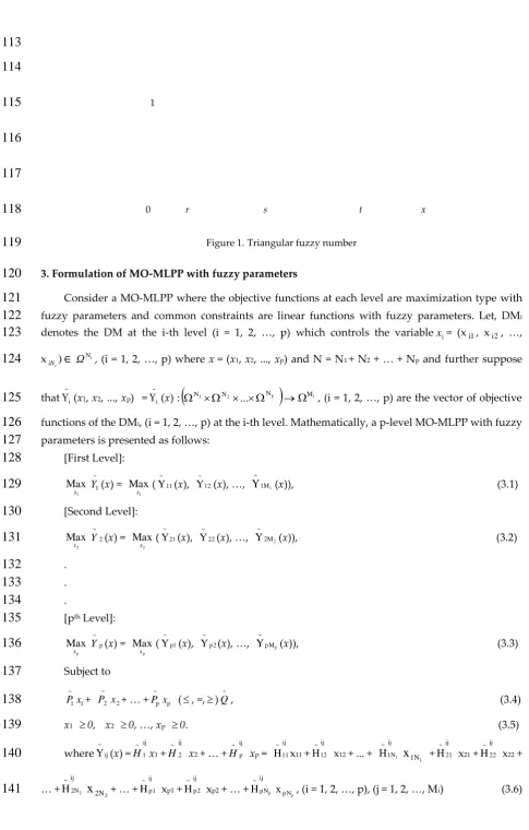
Generally, a triangular fuzzy number is represented as (r, s, t) (see Fig. 1).

109

110

) ( μ~

T x

111

(4)

113

114

1

115

116

117

0 r s t x

118

Figure 1.Triangular fuzzy number

119

3. Formulation of MO-MLPP with fuzzy parameters

120

Consider a MO-MLPP where the objective functions at each level are maximization type with

121

fuzzy parameters and common constraints are linear functions with fuzzy parameters. Let, DMi

122

denotes the DM at the i-th level (i = 1, 2, …, p) which controls the variablexi= (xi1, xi2, …,

123

x )

i

iN i

N

∈ Ω , (i = 1, 2, …, p) where x = (x1, x2, ..., xp) and N = N1 + N2+ … + Np and further suppose

124

that ~

i

 (x1, x2, ..., xp) =

~

i

 (x) :



N1N2  Np





... Mi_{, (i = 1, 2, …, p) are the vector of objective}

125

functions of the DMi, (i = 1, 2, …, p) at the i-th level. Mathematically, a p-level MO-MLPP with fuzzy

126

parameters is presented as follows:

127

[First Level]:

128

1

Max

x

~

1 Y (x) =

1

Max

x ( 11

~

Y (x), 12 ~

Y (x), …, 1M1 ~

Y (x)), (3.1)

129

[Second Level]:

130

2

Max

x 2

~ Y (x) =

2

Max

x ( 21

~

Y (x), 22 ~

Y (x), …, 2M2 ~

~ Y (x) =

p Max

x ( p1

~

Y (x), p 2 ~

Y (x), …, p Mp ~

Y (x)), (3.3)

136

Subject to

137

1 ~

1x

P + 2 ~

2 x

P + … + p

~

px

P (, =,) ~

Q, (3.4)

138

x1 0, x2 0, …, xp 0. (3.5)

139

where ij ~

Y (x) = ij

1 ~ H x1 +

ij

2 ~

H x2+ … +

ij

p ~ H xp =

ij

11 ~

H x11 +

ij

12 ~

H x12 + ... +

ij 1N ~

1 H

1

1N

x

+

ij

21 ~

H x21 +

ij

22 ~

H x22 +

140

… +

ij 2N ~

2

H

2

2N

x

+ … +

ij

p 1 ~

H xp1 +

ij

p 2 ~

H xp2+ … +

ij

p N ~

p H

p p N

x , (i = 1, 2, …, p), (j = 1, 2, …, Mi) (3.6)

(5)

Here, ~

i

P is M  Ni matrix, (i = 1, 2, …, p),

~

Q is the M component column

142

vector. ij

k ~

H = H ,H ,...,H ,

ij kN ~ ij k2 ~ ij k1 ~

k

  

 

(i = 1, 2, …, p), (j= 1, 2, …, Mi) are constants, x = x1x2 … xp is the

143

set of decision vector, N = N1 + N2+…+ Np = total number of decision variables in the system and M is

144

the total number of system constraints. Here, 1 ~

Y (x), 2 ~

Y (x), …, p ~

Y (x) are linear and bounded with

145

fuzzy coefficients and let us represent the system constraints (3.4) & (3.5) as J().

146

4. Deterministic formulation of MO-MLPP with fuzzy parameters

147

At first, we convert the fuzzily described objectives and constraints to deterministic objectives

148

and constraints for a specific value of λ.Now, for specific value ofλ,maximization-type objective

149

functionYij( )

~

x , (i = 1, 2, …, p), (j = 1,2, …, Mi) can be replaced by the upper bound of its

λ

-cut i.e.,

150  

U ij ~ λ

Y 

    

x = p

U ij

p ~ λ 2 U ij

2 ~ λ 1 U ij

1 ~

λ₍_H ₎ _x _ ₍_H ₎ _x __..._ ₍_H ₎ _x

, (i = 1, 2, …, p), (j = 1, 2, …, Mi) (4.1)

151

Similarly, minimization-type objective functionYij( )

~

x , (i =1, 2, …, p), (j = 1,2, …, Mi) can be

152

replaced by the lower bound of itsλ-cut i.e.,

153  

L ij ~ λ

     

x

Y = p

L ij

can be modified by the following constraints:

158

j U N

1 j ij

~ λ

x P   _

  

 _ L

i ~ λ

Q 

    

, (i = 1, 2, …, m1) (4.5)

159

L N

1 j ij

~ λ

P 

 _

   

xj 

U

i ~ λ

Q 

    

, (i = m1+1, m1+2, …, m2) (4.6)

160

The fuzzy equality constraints

161

j N

1 j ij

~

x P 

 = i

~

Q , (i = m2+1, m2+2, …, M) (4.7)

162

can be replaced by two equivalent inequality constraints as given below.

163

U N

1 j

ij ~ λ

P   _

   

xj 

L

i ~ λ

Q 

    

, (i = m2+1, m2+2, …, M) (4.8)

164

L N

1 j ij

~ λ

P 

 _

   

xj 

U

i ~ λ

Q 

    

, (i = m2+1, m2+2, …, M) (4.9)

(6)

Lee and Li [32] proved that the Eq. (4.7) is equivalent to the Eq. (4.8) and Eq. (4.9).

166

Then, for a prescribed value ofλ, the MO-MLPP reduces to the following problem as given

167

below.

168

U 1 ~ λ

)) ( ( Max

1

x Y

x =Max (Y ( )) , (Y ( )) ,..., (Y ( )) ,

U 1M ~ λ U 12 ~ λ U 11 ~ λ

1 1

   

 

x x

x

169

, )) ( Y ( ,..., )) ( Y ( , )) ( Y ( Max ))

( (

Max 2M U

~ λ U 22 ~ λ U 21 ~ λ U

2 ~ λ

2 2

2

   

 

 x x x

x Y

x

170

.

171

.

172

.

173

U p ~

λ₍ ₍ ₎₎

Max p

x Y

x = 

 



 U

pM ~ λ U p2 ~ λ U p1 ~ λ

)) ( Y ( ,..., )) ( Y ( , )) ( Y (

Max p

p

x x

x

174

Subject to

175

U N

1 j ij

~ λ

P 

 _

   

xj 

L

i ~ λ

Q 

    

, (i = 1, 2, …, m1, m2+1, m2+2, …, M)

176

L N

1 j ij

~ λ

P 

 _

   

xj 

U

i ~ λ

Q 

    

, (i = m1+1, …, m2, m2+1, m2+2, …, M)

177

x1



0, x2



0, …, xp



0. (4.10)

178

5. Some basic concepts concerning distance measures

179

Basic concept of distance measure is presented in this section, for additional details see [26, 27,

180

28]. Let, ~

Y(x) = ( 1

~

Y (x), 2

~

Y (x), …, M

~

Y (x)) be the vector of the objective functions with fuzzy

181

parameters. For a prescribed value ofλ, we assume that Y* _{= (} *

1

Y ,Y2*, ..., * M

Y ) be the PIS of the

182

objective functions such that * i

Y = U

i ~ λ

J ( ( ))

Max Y x

x , (i = 1, 2, ..., M) and Y

- _{= (} 

1

Y ,Y2, ..., -M

Y ) be the NIS

183

of the objective functions such thatYi=

L i ~ λ

J ( ( ))

Min Y x

x , (j = 1, 2, ..., M). B

K-metric is used to attain the

184

measure of “closeness”. BK-metric defines the distance between

~

Z(x) and Z*_{which is presented as}

185

follows:

186

Bk =

k 1 M

1 j

k U j ~ λ * j k

j ( ( ))

ε

    

  

   



 _



 Y Y x , k = 1, 2, ..., ∞. (5.1)

187

Here, k j

ε , (j = 1, 2, ..., M; k = 1, 2, ..., ∞) denotes the relative weight of the j-th objective function.

188

However, if U j ~ λ₍_Y ₍_x₎₎

, (j = 1, 2, ..., M) is not expressed in commensurable unit, then we can employ

189

(7)

Bk =

k 1

M

1 j

k

j * j

U j ~ λ * j k j

Y Y

)) ( ( Y ε

    

    

  

 

  

 

 



 

x Y

, k = 1, 2, ..., ∞. (5.2)

191

In order to find the compromise solution of the multi-objective decision making (MODM)

192

problem we solve the following problem:

193

Max ~

Y(x) = ( 1 ~

Y (x), 2 ~

Y (x), …, M ~

Y (x))

194

Subject to

195

1 ~

1x

P + 2

~

2 x

P + … + p

~

px

P (, =,) ~

Q,

196

x1 0, x2 0, …, xp 0. (5.3)

197

According to Lai et al. [33], the above problem (5.3) is transformed into the following auxiliary

198

problem as given below.

199

Min Bk =

k 1

M

1 j

k

j * j

U j ~ λ * j k j

Y Y

)) ( ( Y ε

    

    

  

 

  

 

 



 

x Y

, k = 1, 2, ..., ∞

200

Subject to

201

1 ~

1x

P + 2

~

2 x

P + … + p

~

px

P (, =,)Q~ ,

202

x1 0, x2 0, …, xp 0. (5.4)

203

The parameter ‘k’ is known as the ‘balancing factor’ between the group utility and maximal

204

individual regret. It is to be noted that if the value of ‘k’ increases, the group utility i.e. Bk decreases

205

[33].

206

6. TOPSIS based FGP approach for MO-MLPP with fuzzy parameters

207

For specific value of ofλ, consider the deterministic MODM problem at i-th level is expressed

208

as follows:

209

U i ~ λ

)) ( ( Max

i

x Y

x = 

 



 U

iM ~ λ U i2 ~ λ U i1 ~ λ

)) ( Y ( ,..., )) ( Y ( , )) ( Y (

Max i

i

x x

x

x , (i = 1, 2, …, p)

210

Subject to

211

U N

1 j ij

~ λ

P 

 _

   

xj 

L

i ~ λ

Q 

    

, (i = 1, 2, …, m1, m2+1, m2+2, …, M)

212

L N

1 j ij

~ λ

P   _

   

xj 

U

i ~ λ

Q 

    

, (i = m1+1, …, m2, m2+1, m2+2, …, M)

213

x1 0, x2 0, …, xp 0. (6.1)

214

TOPSIS model for i-th level DM can be formulated as follows:

215

Min (dPISi( ))

k λ

x , (i = 1, 2, …, p)

216

Max (dNISi( ))

k λ

(8)

Subject to

218

U N 1 j ij ~ λ P   _    

xj 

L i ~ λ Q      

, (i = 1, 2, …, m1, m2+1, m2+2, …, M)

219

L N 1 j ij ~ λ P   _    

xj 

U i ~ λ Q      

, (i = m1+1, …, m2, m2+1, m2+2, …, M)

220

x0 0, x1 0, …, xp 0. (6.2)

221

where (gPISi( ))

k λ

x =

k 1 M 1 j k -ij λ * ij λ U ij ~ λ * ij λ k j i ) (Y ) (Y )) ( Y ( ) (Y ε                         x

, (i = 1, 2, …, p);

222

)) ( (gNISi

k λ x = k 1 M 1 j k -ij λ * ij λ -ij λ U ij ~ λ k j i ) (Y ) (Y ) (Y -)) ( Y ( ε                        x

, (i = 1, 2, …, p).

223

Here, * ij λ_(Y ₎

= J Max  x U ij ~ λ₍_Y ₍_x₎₎

and -ij λ ) (Y = J Min  x U ij ~ λ₍_Y ₍_x₎₎

, (i = 1, 2, …, p) are the PIS and

224

NIS for i-th level DM respectively.

225

Let,

 

PIS * k λ i g = J Min 

x (g ( ))

i PIS k λ

x and

The membership functions for (gPISi( ))

k λ

x and (gNISi( ))

k λ

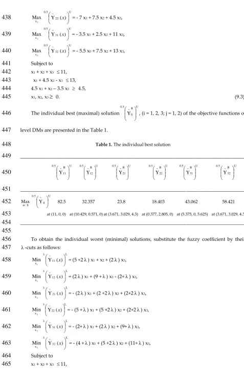
x (see Fig.2) can be constructed as

228

follows:

229

)) ( μ ( PISi

k g λ x =

 

   





 

                  * PIS k λ PIS k λ PIS k λ PIS k λ * PIS(F) k λ * PIS k λ PIS k λ PIS k λ PIS k λ PIS k λ PIS k λ i i i i i i i i i i g )) ( g ( if 1, , g )) ( g ( g if , g g )) ( g ( g )) ( (g g if 0, x x x x

(i = 1, 2, …, p) (6.3)

230

)) ( μ ( NISi

k g λ x =



  

 

   

 

                 * NIS k λ NIS k λ * NIS k λ NIS k λ NIS k λ NIS k λ * NIS k λ NIS k λ NIS k λ NIS k λ NIS k λ i i i i i i i i i i g )) ( g ( if 1, g )) ( g ( g if , g g g -)) ( (g g ) ( g if 0, x x x x

, (i = 1, 2, …, p) (6.4)

231

232

233

μgPISq (x), ( )

μ NIS q

g x Max - Min solution

234

235

1

(9)

PIS q

239

Figure 2. The membership functions of gqPIS(x), NIS q

g (x)

240

Convert the non-linear membership functions (μ PISi( ))

k g λ

x and (μ NISi( ))

k g λ

x , (i = 1, 2, …, p) into

241

equivalent linear membership functions (μ~ PISi( ))

k g λ

x and (μ~ NISi( ))

k g λ

x , (i = 1, 2, …, p) respectively using

242

first order Taylor polynomial series approximation as given below.

243

)) ( μ ( PISi

k g λ

x

~

 (μ PISi( *))

k PIS g λ

x + i(x x_PIS*)

ij N 1 j ij    * PIS i PIS k at ij g λ x )) ( μ ( x x x           

= (μ~ PISi( ))

k g λ

x , (i = 1, 2, …, p) (6.5)

244

where PIS*

x = (x₁PIS*,x₂PIS*,...,x_pPIS*)is such that (μ PISi( *))

k PIS g λ x = J Max 

x (μ i( ))

PIS k g λ

x , (i = 1, 2, …, p);

245

)) ( μ ( NISi

k g λ

x

~

 (μ NISi( *))

k NIS g λ

x + (x x )

* i NIS ij N 1 j ij    * NIS i NIS k at ij g λ x )) ( μ ( x x x           

= (μ~ NISi( ))

k g λ

x , (i = 1, 2, …, p) (6.6)

246

where _xNIS*_{= (}

) ..., , , * * * _NIS p NIS 2 NIS

If PIS* i

β > 1, then we consider PIS* i

β = 1, (i = 1, 2, ..., p) since the value of the membership function

253

cannot be superior than one. Also if PIS* i

α < 0, then we consider PIS* i

α = 0, (i = 1, 2, ..., p) because the

254

value of the membership function cannot be less than zero [30]. The results also hold

255

for NIS* i

β and NIS* i

α , (i = 1, 2, ..., p).

256

(10)

Max (μ PISi( ))

k g λ

x , (i = 1, 2, ..., p)

258

Max (μ NISi( ))

k g λ

x , (i = 1, 2, ..., p)

259

Subject to

260

U N

1 j ij

~ λ

P 

 _

   

xj 

L

i ~ λ

Q 

    

, (i = 1, 2, …, m1, m2+1, m2+2, …, M)

261

L N

1 j

ij ~ λ

P   _

   

xj 

U

i ~ λ

Q 

    

, (i = m1+1, …, m2, m2+1, m2+2, …, M)

262

x1 0, x2



0, …, xp



0. (6.9)

263

According to Pramanik and Dey [22], the flexible membership goals of with aspiration level

264

unity can be expressed as follows:

265

)) ( μ ( PISi

k g λ

x + -PISi

d = 1, (i = 1, 2, ..., p) (6.10)

266

)) ( μ ( NISi

k g λ

x + -NISi

d = 1, (i = 1, 2, ..., p) (6.11)

267

where -PISi

d [0, 1] and -NISi

d [0, 1], (1, 2, …, p) are the negative deviational variables

268

corresponding to PIS and NIS respectively. The following MODM model is solved based on FGP

269

method to achieve the optimal decision of each level DM as follows:

270

271

MODM Model:

272

Min ζ

273

Subject to

274

)) ( μ ( PISi

k g λ

x + -PISi

d = 1, (i = 1, 2, ..., p)

275

)) ( μ ( NISi

k g λ

x + -NISi

d = 1, (i = 1, 2, ..., p)

276

U N

1 j ij

~ λ

P 

 _

   

xj 

L

i ~ λ

Q 

    

, (i = 1, 2, …, m1, m2+1, m2+2, …, M)

277

L N

1 j

ij ~ λ

P   _

   

xj 

U

i ~ λ

Q 

    

, (i = m1+1, …, m2, m2+1, m2+2, …, M)

278

ζ  -PISi d ,ζ 

-NISi

d , (i = 1, 2, ...,p)

279

-PISi

d [0, 1], -NISi

d [0, 1], (i = 1, 2, ..., p)

280

x1



0, x2



0, …, xp



0. (6.12)

(11)

Solving the above Eq. (6.12), let i

x = ( i 1

x , i 2

x , …, i p

x ) be the optimal solution of i-th level DM.

282

To avoid any unwanted circumstance i.e decision deadlock, the level DMs should offer some

283

relaxation on decision by assigning preference upper and lower bounds on the decision variables

284

under their control [18, 22, 30, 35, 36, 37] for ovallall benefit and smooth functioning of the

285

organization and these preference bounds are included in the constraints set.

286

Consider i i



and i i



, (i = 1, 2, ..., p) be the lower and upper tolerance values on the decision vector

287

considered by i-th level DM such that

288



i i

x -



ii  i i

x  xii+ i i



, (i = 1, 2, ..., p) (6.13)

289

Therefore, the new hybrid models of FGP and TOPSIS for MO- MLPP for a specificλcan be

290

formulated as follows:

291

Model (I):

292

Minimize ρ

293

Subject to

294

)) ( μ ( PISi

k g λ

x + -PISi

D = 1, (i = 1, 2, ..., p)

295

)) ( μ ( NISi

k g λ

x + -NISi

D = 1, (i = 1, 2, ..., p)

296

U N

1 j ij

~ λ

P 

 _

   

xj 

L

i ~ λ

Q 

    

, (i = 1, 2, …, m1, m2+1, m2+2, …, M)

297

L N

1 j ij

~ λ

P   _

   

xj 

U

i ~ λ

Q 

    

, (i = m1+1, …, m2, m2+1, m2+2, …, M)

298



i i

x -



ii i i

x  xii+ i i



, (i = 1,2, ...,p)

299

ρ  -PISi

D ,ρ  -NISi

D , (i = 1,2, ...,p)

300

-PISi

D [0, 1], -NISi

D [0, 1], (i = 1,2, ...,p)

301

x1 0, x2 0, …, xp 0. (6.14)

302

303

304

Model (II):

305

Minimizeσ= -PIS PISiD i

w +

-NIS NISiD i

w , (i = 1, 2, ...,p)

306

Subject to

307

)) ( μ ( PISi

k g λ

x + -PISi

D = 1, (i = 1, 2, ..., p)

308

)) ( μ ( NISi

k g λ

x + -NISi

(12)

U N

1 j ij

~ λ

P 

 _

   

xj 

L

i ~ λ

Q 

    

, (i = 1, 2, …, m1, m2+1, m2+2, …, M)

310

L N

1 j ij

~ λ

P   _

   

xj 

U

i ~ λ

Q 

    

, (i = m1+1, …, m2, m2+1, m2+2, …, M)

311



i i

x - i i



 i i

x  xii+ i i



, (i = 1, 2, ...,p)

312

-PISi

D [0, 1], -NISi

D [0, 1], (i = 1,2, ...,p)

313

x1 0, x2 0, …, xp 0. (6.15)

314

The i-th level DM can take the normalized weight i.e. i PIS

w + i

NIS

w = 1, (i = 1, 2, ..., p) or any

315

preference weight in the decision making situation. -PISi

D and -NISi

D [0, 1], (i = 1, 2, ..., p) are

316

negative deviational variables.

317

7. Selection of compromise optimal solution of MO-MLPP

318

For selecting compromise optimal solution, we consider a termination criteria based on distance

319

functios. The family of distance functions defined by Zeleny [38] is expressed as given below.

320

L(

ω

, q) =







 



 _ 1

K

1

k ωq(1 q) (7.1)

321

whereq, (q = 1, 2, ..., Q) represents the measure of closeness of the preferred compromise

322

solution to the optimal compromise solution vector regarding q - th objective function. Here, ω=

323

(ω1,ω2, ..., ωQ) denotes the vector of attribute level and(1_  _ ) is the distance parameter.

324

We consider= 2, then the distance function becomes

325

L2 (

ω

, q) =

2 1 Q

1 q

2 q 2

q(1 )

ω _

 

 _ _

  (7.2)

326

For maximization type of problemq = (the preferred compromise solution/ the individual best

327

solution). The solution for which L2 (

ω

, q) will be minimal would be the compromise optimal

328

solution for each level DM.

329

330

331

8 TOPSIS based algorithm to MO-MLPP with fuzzy parameters

332

The proposed TOPSIS based algorithm (see Fig 3) for MO-MLPP with fuzzy parameters is

333

provided below.

334

Step 1: For specified value ofλ, the upper and lower bounds of the fuzzily described objective

335

(13)

Step 2: Calculate the maximum and minimum values for the upper and lower λ- cuts of the

337

objective functions for all level DMs separately subject to the common constraints.

338

Step 3: Compute PIS and NIS for i-th level DM and formulate distance functions for PIS and

339

NIS (gPISi( ))

k λ

x , (i = 1, 2, ..., p).

344

Step 6: Transform the non-linear membership functions (μ PISi( ))

k g λ

x and (μ NISi( ))

k g λ

x , (i = 1, 2, ..., p)

345

into equivalent linear membership functions (μ~ PISi( ))

k g λ

x and (μ~ NISi( ))

k g λ

x , (i = 1, 2, ..., p) respectively

346

by using suitable transformation technique and then normalize equivalent linear membership

347

functions.

348

Step 7: Formulate the MODM model (6.12) to identify the satisfactory solution i

x = ( i 1

x , i 2

x ,

349

…, i p

x ) , (i = 1, 2, ..., p) of i-th level DM.

350

Step 8: DMs offer the lower and upper tolerance values



iiand i i



, (i = 1,2, ...,p) respectively on

351

the decision vector i

x = ( i 1

x , i 2

x , …, i p

x ) , (i = 1, 2, ..., p).

352

Step 9: Construct the TOPSIS based FGP Models (6.14) and (6.15).

353

Step 10: Solve the Models (6.14) and (6.15).

354

Step 11: L2 (

ω

, q) is employed to identify better compromise optimal solution of the problem.

355

Step 12: If the compromise optimal solution is acceptable to all level DMs then stop. Otherwise,

356

adjust the lower and upper tolerance values of all level DMs and go to Step 8.

357

358

359

360

361

362

363

364

365

366

367

368

369

Start _{Each level DM provides his/her fuzzily described objective functions}

Fuzzily described constraints are given

Upper and lower bounds of the fuzzily described objective

functions and constraints are defined for specific value of λ

(14)

370

371

372

373

374

375

376

377

378

379

380

381

382

383

384

385

386

387

388

389

390

391

392

393

394

395

396

397

398

399

400

401

A flowchart of the proposed algorithms

402

9. Numerical example

403

The following MO-MLPP with fuzzy parameters is considered to demonstrate the proposed

404

procedure.

405

[First Level]

406

1 x

Max( 11 ~

Y (x) = ~

7x1 + x2 +

~

2x3, 12 ~

Z (x) = ~

2x1 +

~

10 x2

-~

3x3)

407

[Second Level]

408

2 x

Max( 21 ~

Y (x) = -~

2x1 +

~

4x2 +

~

4x3, 22 ~

Z (x) = -6~x1 +

~

7x2 +

~

4x3),

(15)

[Third Level]

410

3 x

Max( 31 ~

Y (x) = -3~x1 +

~

2x2 +

~

10x3, 32 ~

Z (x) = -5~x1 +

~

7x2 +

~

12x3)

411

Subject to

412

~

2x1 +

~

2x2 + x3 

~

10,

413

x1 +

~

5x2 -

~

2x3 

~

12,

414

~

4x1 + x2 -

~

3x3 

~

~

2= (0, 2, 3), 3~= (2, 3, 4), 4~= (2, 4, 5), 5~= (4, 5, 6), 6~= (5, 6, 8), 7~= (5, 7, 8), 10~ = ( 9, 10, 12), 12~ =

418

(11, 12, 14).

419

  

 

x = - (6 - λ) x0 + (8 - λ) x2 + (14 - 2λ) x3,

427

Subject to

428

(2λ) x1 + (2λ) x2 + x3 (12 - 2λ),

429

x1 + (4 +λ) x2 - (2λ) x3 (14 - 2λ),

430

(5 - λ) x1 + x2– (4 - λ) x3  (4 +λ),

431

x1, x2, x3 0. (9.2)

432

  

 

x = - 2.5 x1 + 4.5 x2 + 4.5 x3,

(16)

2 x

Max

U

22 ~ 0.5

) (

Y 

  

 

x = - 7 x1 + 7.5 x2 + 4.5 x3,

438

3 x

Max

U

31 ~ 0.5

) (

Y 

  

 

x = - 3.5 x1 + 2.5 x2 + 11 x3,

439

3 x

Max

U

32 ~ 0.5

) (

Y 

  

 

x = - 5.5 x0 + 7.5 x2 + 13 x3,

440

Subject to

441

x1 + x2 + x3 11,

442

x1 + 4.5 x2 - x3 13,

443

4.5 x1 + x2– 3.5 x3  4.5,

444

x1, x2, x3



0. (9.3)

445

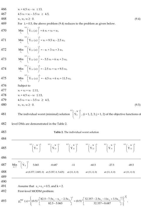
The individual best (maximal) solution

U B

ij ~ 0.5

Y _

    

, (i = 1, 2, 3; j = 1, 2) of the objective functions of

446

level DMs are presented in the Table 1.

447

Table 1.The individual best solution

448

________________________________________________________________________________________

449

U B

11 ~ 0.5

Y _

    

U B

12 ~ 0.5

Y _

    

U B

21 ~ 0.5

Y _

    

U B

22 ~ 0.5

Y _

    

U B

31 ~ 0.5

Y _

    

U B

32 ~ 0.5

Y _

    

450

__________________________________________________________________________________________________

451

S Max



x

U

ij ~ 0.5

Y 

    

82.5 32.357 23.8 18.403 43.062 58.421

452

at (11, 0, 0) at (10.429, 0.571, 0) at (3.671, 3.029, 4.3) at (0.377, 2.805, 0) at (5.375, 0, 5.625) at (3.671, 3.029, 4.3)

453

__________________________________________________________________________________________________

454

455

  

 

x = - (4 +λ) x1 + (5 +2λ) x2 + (11+λ) x3,

463

Subject to

464

x1 + x2 + x3 11,

(17)

x1 + 4.5 x2 - x3 13,

466

4.5 x1 + x2– 3.5 x3  4.5,

467

x1, x2, x3



0. (9.4)

468

For λ= 0.5, the above problem (9.4) reduces to the problem as given below.

469

1 x Min L 11 ~ 0.5 ) ( Y      

x = 6 x1 + x2 + x3,

470

1 x Min L 12 ~ 0.5 ) ( Y      

x = x1 + 9.5 x2 - 2.5 x3,

471

2 x Min L 21 ~ 0.5 ) ( Y      

x = - x1 + 3 x2 + 3 x3,

472

2 x Min L 22 ~ 0.5 ) ( Y      

x = - 5.5 x1 + 6 x2 + 3 x3,

473

3 x Min L 31 ~ 0.5 ) ( Y      

x = - 2.5 x1 + x2 + 9.5 x3,

474

3 x Min L 32 ~ 0.5 ) ( Y      

x = - 4.5 x1 + 6 x2 + 11.5 x3,

475

Subject to

476

x1 + x2 + x3



11,

477

x1 + 4.5 x2 - x3



13,

478

4.5 x1 + x2– 3.5 x3



4.5,

479

x1, x2, x3



0. (9.5)

480

The individual worst (minimal) solution

L W ij ~ 0.5 Y _     

, (i = 1, 2, 3; j = 1, 2) of the objective functions of

481

level DMs are demonstrated in the Table 2.

482

Table 2.The individual worst solution

483

________________________________________________________________________________________

484

L W 11 ~ 0.5 Y _      L W 12 ~ 0.5 Y _      L W 21 ~ 0.5 Y _      L W 22 ~ 0.5 Y _      L W 31 ~ 0.5 Y _      L W 32 ~ 0.5 Y _     

485

__________________________________________________________________________________________________

486

J Min  x L ij ~ 0.5 Y      

5.065 -8.687 -11 -60.5 -27.5 -49.5

487

at (0.377, 2.805, 0) at (5.357, 0, 5.625) at (11, 0, 0) at (11, 0, 0) at (11, 0, 0) at (11, 0, 0)

488

__________________________________________________________________________________________________

489

490

Assume that ε1=ε2= 0.5, and k = 2.

491

First-level MODM problem:

492

) ( gPIS1

2 x = ,

(18)

) ( gNIS1

2 x =

2 1 2 3 2 1 2 2 3 2 1 2 687 . 8 357 . 2 3 687 . 8 3.5x x 11 2.5x ) 5 . 0 ( 065 . 5 5 . 82 5.065 -2.5x x 7.5x ) 5 . 0 (                            

494

We determine:



PIS



* 2 ( )

g 1 x = J Min  x 1 PIS 2

g (x) = 0.022 at (10.509, 0.491, 0);



gPIS2 1(x)



= J Max  x 1 PIS 2

g (x) =

495

0.606 at (1, 0, 0);



NIS



* 2 ( )

g 1 x = J Max  x 1 NIS 2

g (x) = 0.69 at (10.429, 0.571, 0);



gNIS2 1(x)



= J Min  x 1 NIS 2

g (x) = 0.134 at

496

(1.415, 0, 0.533).

497

The membership functions of PIS1 2

g (x) and NIS1 2

g (x) can be formulated as follows:

498

              022 . 0 ) ( g if 1, 606 . 0 ) ( g 022 . 0 if , 022 . 0 606 . 0 ) ( g 606 . 0 ) ( g 0.606 if 0, ) ( μ 1 1 1 1 1 PIS 2 PIS 2 PIS 2 PIS 2 PIS 2 g x x x x x ;

499

) ( μ NIS1

2

g x =

(-0.036) +

-NISi

d = 1,

505

α  -PIS1 d ,α

-NIS1

d ,

506

-PIS1

d [0, 1], -NIS1

d [0, 1],

507

x1 + x2 + x3 11,

508

x1 + 4.5 x2 - x3 13,

509

4.5 x1 + x2– 3.5 x3  4.5,

510

x1, x2, x3



0. (9.6)

511

The satisfactory solution of the First-level MODM problem is obtained as F* x = ( F*

1

x , F* 2

x , F* 3

x ) =

512

(10.429, 0.571, 0). Suppose the First-level DM decides F* 1

x = 10.429 with lower tolerance 1 1



= 5.929

513

and upper tolerance 1 1

 = 0.571 such that 10.429 – 5.929 x1 10.429 + 0.571.

514

(19)

) (

gPIS2 2 x = ,

5 . 60 403 . 18 4.5x x 5 . 7 7x 403 . 18 ) 5 . 0 ( 11 8 . 23 4.5x x 5 . 4 2.5x 8 . 3 2 ) 5 . 0 ( 2 1 2 3 2 1 2 2 3 2 1 2                         

516

) ( gNIS2 1 x =

2 1 2 3 2 1 2 2 3 2 1 2 5 . 60 403 . 18 5 . 60 4.5x x 5 . 7 7x -) 5 . 0 ( 11 8 . 23 11 4.5x x 5 . 4 2.5x -) 5 . 0 (                             

517

We calculate:



gPIS2 ( )



* 2 x = J Min  x 2 PIS 2

g (x) = 0.013 at (3.653, 3.027, 4.276);



gPIS2 2(x)



g (x) =

518

0.953 at (11, 0, 0);



gNIS2 ( )



* 2 x = J Max  x 2 NIS 2

g (x) = 0.698 at (3.671, 3.029, 4.3);



g2NIS1(x)



= J Min  x 2 NIS 2

g (x) =

519

0.054 at (8.96, 0, 2.04).

520

The membership functions PIS2 2 g

μ (x) and NIS2 2 g

μ (x) can be obtained as follows:

521

522

) ( μ _NIS2

2

g x =

0.036 +

-PIS2

d = 1,

528

1 + (x1 – 3.671)



(-0.088) + (x2 – 3.029)



0.123 + (x3 – 4.3)



0.103 +

-NIS2 d = 1,

529

α  -PIS2

d ,α -NIS2 d ,

530

-PIS1

d [0, 1], -NIS2

d [0, 1],

531

x1 + x2 + x3 11,

532

x1 + 4.5 x2 - x3 13,

533

4.5 x1 + x2– 3.5 x3  4.5,

534

x1, x2, x3



0. (9.7)

535

The satisfactory solution of the Second-level MODM problem is determined as S* x =

536

( S* 1

x , S* 2

x , S* 3

x ) = (3.672, 3.027, 4.3). Let the Second-level DM decides S* 2

x = 3.027 with lower tolerance

537

2 2

 = 1.027 and upper tolerance22= 1.473 such that 3.027 – 1.027



x2



3.027 + 1.473.

(20)

Third-level MODM problem:

539

) (

gPIS2 3 x = ,

5 . 49 421 . 58 x 2 1 x 5 . 7 5.5x 421 . 58 ) 5 . 0 ( 5 . 27 062 . 43 9.5x x 2.5x 062 . 3 4 ) 5 . 0 ( 2 1 2 3 2 1 2 2 3 2 1 2                             

540

) ( gNIS₂ 3 x =

*

2 ( )

g 3 x = J Max  x 3 NIS 2

g (x) = 0.625 at (3.671, 3.029, 4.3);



gNIS3( )





2 x =

J Min  x 3 NIS 2

d (x) = 0.02 at (10.241,

543

0.613, 0).

544

The membership functions of PIS3 2

g (x) and NIS3 2

g (x) can be presented as given below.

545

546

) ( μ _NIS3

2

g x =

0.125) – 0.072)/ (1-0.072) +

-PIS3

d =

552

1,

553

1 + (x1 – 3.671)



(-0.049) + (x2 – 3.029)



0.048 + (x3 – 4.3)



0.137 +

-NIS3 d = 1,

554

α  -PIS3

0. (9.8)

560

By solving the above Eq. (9.8), the satisfactory solution of the Third-level DM is obtained as T* x =

561

( T* 1

x , T* 2

x , T* 3

(21)

decides T* 3

(-0.002) – 0.004)/ (1-0.004)) +

-PISi D = 1,

-PIS3 D =

574

1,

575

1 + (x1 – 3.671)



(-0.049) + (x2 – 3.029)



0.048 + (x3 – 4.3)



0.137 + D-_NIS3= 1,

576

ρ  -PISi

D ,ρ  -NISi

D , (i = 1, 2, 3)

577

-PISi

D [0, 1], -NISi

D [0, 1], (i = 1, 2, 3)

578

x1 + x2 + x3 11,

579

x1 + 4.5 x2 - x3 13,

580

4.5 x1 + x2– 3.5 x3  4.5,

581

10.429 – 5.929  x1 10.429 + 0.571,

582

3.027 – 1.027  x2 3.027 + 1.473,

583

4.3 – 2.3



x3



4.3 + 0.7,

584

x1, x2, x3



0. (9.10)

585

The optimal solution of the Model (I) for MO-MLPP is shown in the Table 3.

586

587

588

Table 3. The optimal solution of Model (I)

589

__________________________________________________________________________________________________

590

Approach Optimal solution Optimal solution point Objective values Membership values

591

Model (I)

ρ

= 0.3550353 4.963, 2.559, 3.478 48.475, 28.384, 14.759, 0.561, 0.903, 0.74,

592

0.102, 27.285,37.11 0.768, 0.776, 0.802

593

(22)

Model (II)

595

Minimizeσ=1/6( -PISi

D +

-NISi

598

1 + (x1 – 10.429)



0.1 + (x2 – 0.571)



0.183 + (x3 – 0)



(-0.036) +

-NISi D = 1,

599

1 + (x1 – 3.653)



(-0.05) + (x2 – 3.027)



0.557 + (x3 – 4.276)



0.036 +

604

-PISi

D



[0, 1], -NISi

D



[0, 1], (i = 1, 2, 3)

605

x1 + x2 + x3 11,

606

x1 + 4.5 x2 - x3 13,

607

4.5 x1 + x2– 3.5 x3  4.5,

608

10.429 – 5.929  x1 10.429 + 0.571,

609

3.027 – 1.027  x2 3.027 + 1.473,

610

4.3 – 2.3  x3 4.3 + 0.7,

611

x1, x2, x3



0. (9.11)

612

Here, we consider the normalized weights associated with negative deviational variables. The

613

optimal solution of Model (II) is shown in the Table 4.

614

Table 4. The optimal solution of Model (II)

615

________________________________________________________________________________________

616

Approach Optimal solution Optimal solution point Objective values Membership values

617

Model (II)

σ

= 0.225927 4.5, 2.727, 3.773 45.91, 28.042, 18, 0.527, 0.895, 0.833,

618

5.931, 32.57, 44.752 0.842, 0.851, 0.873

619

620

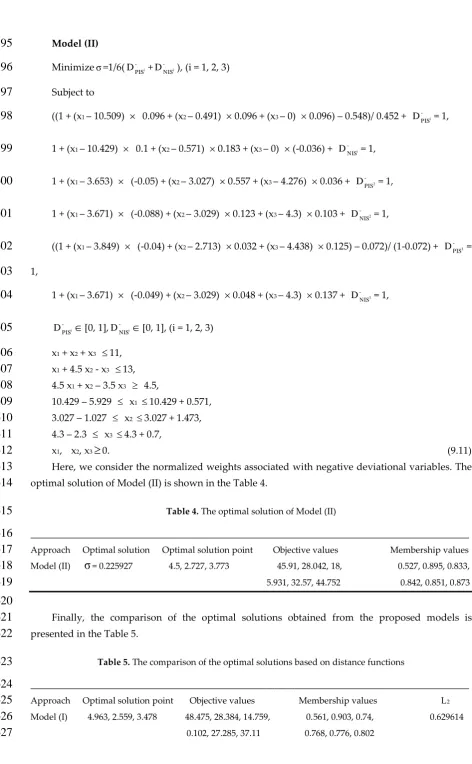
Finally, the comparison of the optimal solutions obtained from the proposed models is

621

presented in the Table 5.

622

Table 5. The comparison of the optimal solutions based on distance functions

623

________________________________________________________________________________________

624

Approach Optimal solution point Objective values Membership values L2

625

Model (I) 4.963, 2.559, 3.478 48.475, 28.384, 14.759, 0.561, 0.903, 0.74, 0.629614

626

0.102, 27.285, 37.11 0.768, 0.776, 0.802