Tuning variable selection procedures by adding noise

(1)

Tuning Variable Selection Procedures by Adding

Noise

Xiaohui Luo,

∗

_{Leonard A. Stefanski and Dennis D. Boos}

†

Abstract

Many variable selection methods for linear regression depend critically on tuning parameters

that control the performance of the method, e.g., “entry” and“stay” significance levels in

forward and backward selection. However, most methods do not adapt the tuning parameters

to particular data sets. We propose a general strategy for adapting variable selection tuning

parameters that effectively estimates the tuning parameters so that the selection method

avoids overfitting and underfitting. The strategy is based on the principle that underfitting and

overfitting can be directly observed in estimates of the error variance after 1) adding controlled

amounts of additional independent noise to the response variable and 2) then running a variable

selection method. It is related to the simulation technique SIMEX found in the measurement

error literature. We focus on forward selection because of its simplicity and ability to handle

large numbers of explanatory variables. Monte Carlo studies show that the new method

compares favorably with established methods.

∗_{Xiaohui Luo is Biometrician, Clinical Biostatistics, Merck Research Laboratories, Rahway, NJ 07065-0900}

(E-mail: edmund [email protected]).

†_{Leonard A. Stefanski and Dennis D. Boos are Professors, Department of Statistics, North Carolina State}

(2)

KEY WORDS: AIC; BIC; Forward selection; Mallows Cp; Model selection; Regression; SIMEX.

1. INTRODUCTION

Common variable selection methods such as stepwise, forward and backward selection, and

gen-eralizations of Mallows Cp (e.g., Atkinson, 1980) depend on tuning parameters that control the

selection procedure, e.g., entry/stay significance levels for stepwise, forward and backward

selec-tion, and a penalty factor for generalized MallowsCp. Depending on the choice of tuning parameter,

the selection procedure may tend to underfit or overfit the model by selecting too few or too many

variables. For example, the default significance level to enter in the SAS forward selection

proce-dure is αEnter = 0.50 and is known to result in overfitting. Conversely, taking αEnter too small will

prevent important predictors from entering the model. Other variable selection procedures have

similar features. Atkinson’s (1980) generalization of Mallows Cp chooses the subset of variables

that minimizes a penalized log-likelihood criterion. The tuning parameter is the penalty for adding

an additional variable to the model. If this penalty is negligible, then unimportant variables will

enter the model at a high rate. If it is too large, then important variables will be restricted from

entering the chosen model.

Some studies provide general guidelines for selecting tuning parameters. For example, based

on simulation results, Atkinson (1980) and Zhang (1992) suggested that the penalty factor for

Atkinson’s generalized Mallows Cp statistic should be chosen between 1.5 and 6 (Mallows Cp is

obtained when the penalty factor is set equal to 2). Forward selection is well discussed in many

(3)

on the use of data-dependent tuning parameters for forward selection and generalized Cp. The

research described in this paper addresses this void. We introduce a generally applicable,

simulation-based method for choosing tuning parameters in variable selection procedures. The new method

exploits the fact that, when coupled with a variable selection procedure, both underfitting and

overfitting result in biased estimates of the error variance. The basic idea is to add controlled

amounts of random error to the response variable and tune the model selection procedure to estimate

the new error variance in an unbiased way. The method is related to the SIMEX (simulation

extrapolation) method used in the measurement error literature to estimate and reduce bias (Cook

and Stefanski, 1994; Stefanski and Cook, 1995; Carroll et al., 1995). In model selection contexts

Breiman (1992) adds random error to the response variable to estimate model error (see definition

below), and Ye (1998) and Shen and Ye (2002) use it to estimate model degrees of freedom.

Following a general introduction and discussion of variable selection in linear models in

Sec-tion 2., the tuning strategy is outlined in general terms and in detail for forward selecSec-tion in

Section 3. The method is extensively studied via simulation in Section 4., and further illustrated

by application to two data sets in Section 5.

2. VARIABLE SELECTION IN LINEAR REGRESSION

Consider the linear regression model

Y =µ+ǫ=X β+ǫ (1)

where Y = (Y1, Y2, . . . , Yn)T is a vector of dependent variables, µ= E(Y) =Xβ, X is a full-rank

design matrix with n observations and pMax predictors, ǫ∼ N(0, σ

2

In) with σ

2

unknown and In

(4)

Henceforth, predictors with nonzero coefficients are called important, those with zero coefficients

are unimportant. If the rows ofX are random, then we are thinking of conditional analyses holding

X fixed.

Two common objectives of variable selection are interpretation and prediction. When statistical

modeling is an adjunct to the development and testing of substantive theoretical models, the

variables that enter the model are important because they often give insight to and sometimes

guide the process of theoretical model development. For such applications of variable selection the

ability to distinguish between important and unimportant variables is paramount. This aspect of

variable selection is not as crucial when prediction is the sole or primary objective of modeling. For

prediction, the utility of the selected model is often evaluated by prediction error (PE), defined as

PE = E(Ynew₋Yb)T(Ynew₋Yb) = ME +n σ2

, (2)

where the expectation is taken only with respect to Ynew, and

ME = (Yb ₋µ)T₍_Y_b

−µ), (3)

whereYb is the least squares estimate ofY,Ynew is a random vector independently and identically

distributed asY, and ME denotes the model error. The expected prediction error is thus determined

by the expected model error given by,

E(ME) = (E(Yb)₋µ)T _(E(_Y_b₎

−µ) +p σ2

, (4)

(5)

purpose of prediction entails a bias-variance tradeoff. Entering more variables generally reduces

bias, but inflates variance.

Many model selection criteria are based on estimating statistical information such as the Akaike

Information Criterion (AIC) and the Bayesian Information Criterion (BIC). The key idea behind

an information criterion is to penalize the likelihood for the model complexity and select a model

by maximizing the penalized likelihood criterion. Under linear regression with normal errors, AIC

is asymptotically equivalent to Mallows Cp statistic, which is a special case of Atkinson’s (1980)

generalized Cp statistic, given by

GMCη(J) =

SSE(J)

σ2 −n+η pJ (5)

whereJ is a subset model,pJ is the number of predictors inJ, SSE(J) is the residual sum of squares

of J, η is the penalty factor for model complexity, and in practiceσ2

is usually estimated by σb2

F,

the residual mean squares from the full model. For given η, a model is selected by minimizing

GMCη(J) over all the subset models. But different models may be selected due to different choices

of penalty factors.

Mallows Cp (η = 2) is used widely and abused as well. It was pointed out by Mallows (1973)

and reemphasized by Mallows (1995) that E(PE) = E(σb2

Cp) if the additive error is independently

distributed with mean 0 and variance σ2

, σb2

is an unbiased estimator of σ2

, and the model is

selected independently of the data under study. But the last assumption is usually conveniently

overlooked in practice. Hence selecting a model by minimizing Cp tends to overfit, a fact which is

manifest in the Monte Carlo study in Section 4.

(6)

mean squares is given by

MSE(J) = Y

T

(In−PJ)Y

n₋pJ

(6)

where In is ann×n identity matrix, and PJ =XJ(XTJ XJ)−1XTJ, the projection matrix of XJ.

IfJ contains all the important variables, (n₋pJ) MSE/σ2follows aχ2n−pJ distribution and hence

E(MSE) = σ2

; we call such models inclusive. Otherwise, (n₋pJ) MSE/σ2 follows a noncentral

χ2

n−pJ distribution with E(MSE) > σ

2

; such models are called non-inclusive. If the coefficients of

the important variables are not too small and the predictors are uncorrelated, then we will have

a very good separation between inclusive models and non-inclusive models. Consequently we can

find the true model by intersecting all the inclusive models.

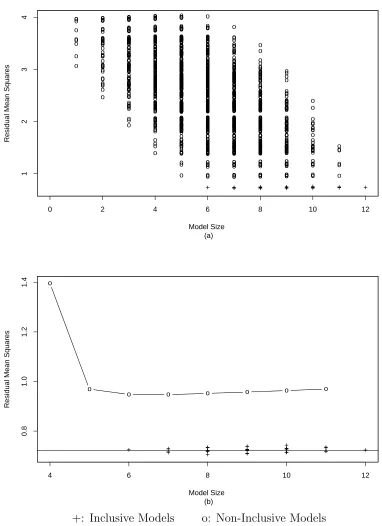
For example, suppose that there are six important variables (with coefficients all equal) among

twelve uncorrelated predictors, and that the error follows a standard normal distribution. The

common value of the coefficients is chosen so that the theoretical R2

= 0.75. In Figure 1 (a), the

MSE of each subset model is plotted versus its model size. All the inclusive models appear at the

bottom of the plot. For model sizes less than six, there is no separation between the models because

all the models are non-inclusive. In Figure 1 (b), the best non-inclusive models (giving minimum

MSE) at each model size _≥ 4 are plotted and connected, and all the inclusive models are plotted

as well. In addition a horizontal line at σb2

F is drawn as a baseline. We see that the models are

well separated. But if the predictors are correlated or some of the coefficients are tiny, then the

noncentral parameter of theχ2

distribution will be very small, and consequently it is more difficult

to distinguish inclusive models from non-inclusive models.

One common approach to model selection is to first identify the model maximizing R2

at each

model size, and then compare MSE of the candidate models with the baseline σb2

F. A model is

(7)

o o o o o o o o o o o o o o o o o o o o o o o o o o o o o o o o o o o o o o o o o o o o o o o o o o o o o o o o o o o o o o o o o o o o o o o o o o o o o o o o o o o o o o o o o o o o o o o o o o o o o o o o o o o o o o o o o o o o o o o o o o o o o o o o o o o o o o o o o o o o o o o o o o o o o o o o o o o o o o o o o o o o o o o o o o o o o o o o o o o o o o o o o o o o o o o o o o o o o o o o o o o o o o o o o o o o o o o o o o o o o o o o o o o o o o o o o o o o o o o o o o o o o o o o o o o o o o o o o o o o o o o o o o o o o o o o o o o o o o o o o o o o o o o o o o o o o o o o o o o o o o o o o o o o o o o o o o o o o o o o o o o o o o o o o o o o o o o o o o o o o o o o o o o o o o o o o o o o o o o o o o o o o o o o o o o o o o o o o o o o o o o o o o o o o o o o o o o o o o o o o o o o o o o o o o o o o o o o o o o o o o o o o o o o o o o o o o o o o o o o o o o o o o o o o o o o o o o o o o o o o o o o o o o o o o o o o o o o o o o o o o o o o o o o o o o o o o o o o o o o o o o o o o o o o o o o o o o o o o o o o o o o o o o o o o o o o o o o o o o o o o o o o o o o o o o o o o o o o o o o o o o o o o o o o o o o o o o o o o o o o o o o o o o o o o o o o o o o o o o o o o o o o o o o o o o o o o o o o o o o o o o o o o o o o o o o o o o o o o o o o o o o o o o o o o o o o o o o o o o o o o o o o o o o o o o o o o o o o o o o o o o o o o o o o o o o o o o o o o o o o o o o o o o o o o o o o o o o o o o o o o o o o o o o o o o o o o o o o o o o o o o o o o o o o o o o o o o o o o o o o o o o o o o o o o o o o o o o o o o o o o o o o o o o o o o o o o o o o o o o o o o o o o o o o o o o o o o o o o o o o o o o o o o o o o o o o o o o o o o o o o o o o o o o o o o o o o o o o o o o o o o o o o o o o o o o o o o o o o o o o o o o o o o o o o o o o o o o o o o o o o o o o o o o o o o o o o o o o o o o o o o o o o o o o o o o o o o o o o o o o o o o o o o o o o o o o o o o o o o o o o o o o o o o o o o o o o o o o o o o o o o o o o o o o o o o o o o o o o o o o o o o o o o o o o o o o o o o o o o o o o o o o o o o o o o o o o o o o o o o o o o o o o o o o o o o o o o o o o o o o o o o o o o o o o o o o o o o o o o o o o o o o o o o o o o o o o o o o o o o o o o o o o o o o o o o o o o o o o o o o o o o o o o o o o o o o o o o o o o o o o o o o o o o o o o o o o o o o o o o o o o o o o o o o o o o o o o o o o o o o o o o o o o o o o o o o o o o o o o o o o o o o o o o o o o o o o o o o o o o o o o o o o o o o o o o o o o o o o o o o o o o o o o o o o o o o o o o o o o o o o o o o o o o o o o o o o o o o o o o o o o o o o o o o o o o o o o o o o o o o o o o o o o o o o o o o o o o o o o o o o o o o o o o o o o o o o o o o o o o o o o o o o o o o o o o o o o o o o o o o o o o o o o o o o o o o o o o o o o o o o o o o o o o o o o o o o o o o o o o o o o o o o o o o o o o o o o o o o o o o o o o o o o o o o o o o o o o o o o o o o o o o o o o o o o o o o o o o o o o o o o o o o o o o o o o o o o o o o o o o o o o o o o o o o o o o o o o o o o o o o o o o o o o o o o o o o o o o o o o o o o o o o o o o o o o o o o o o o o o o o o o o o o o o o o o o o o o o o o o o o o o o o o o o o o o o o o o o o o o o o o o o o o o o o o o o o o o o o o o o o o o o o o o o o o o o o o o o o o o o o o o o o o o o o o o o o o o o o o o o o o o o o o o o o o o o o o o o o o o o o o o o o o o o o o o o o o o o o o o o o o o o o o o o o o o o o o o o o o o o o o o o o o o o o o o o o o o o o o o o o o o o o o o o o o o o o o o o o o o o o o o o o o o o o o o o o o o o o o o o o o o o o o o o o o o o o o o o o o o o o o o o o o o o o o o o o o o o o o o o o o o o o o o o o o o o o o o o o o o o o o o o o o o o o o o o o o o o o o o o o o o o o o o o o o o o o o o o o o o o o o o o o o o o o o o o o o o o o o o o o o o o o o o o o o o o o o o o Model Size (a)

Residual Mean Squares

0 2 4 6 8 10 12

1 2 3 4 + +++ +++++ ++++ +++++ +++ + o o

o o o o o o

Model Size (b)

Residual Mean Squares

4 6 8 10 12

0.8

1.0

1.2

1.4

+ ₊+++ ++++++++₊ ++++++++₊₊₊ +++++₊₊₊ ₊₊₊++ ₊

+: Inclusive Models o: Non-Inclusive Models

(8)

the baseline. The model with the smallest size among the acceptable candidate models is then

selected. This approach is equivalent to applying the same rule on Mallows Cp but using model

size as a baseline, which views Mallows Cp as an estimate of the model size (Mallows 1995). For

subset model J,

Cp =

SSE(J)

b

σ2

F

−(n₋2pJ) = (n−pJ)

MSE(J)

b

σ2

F

−1

+pJ ;

and then, Cp ≤pJ ⇐⇒MSE(J)≤bσ

2

F (7)

We call this approach intelligent Cp and denote it by ICp to distinguish it from the minimum Cp

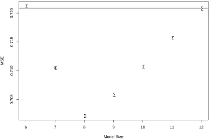
method that selects the model with the smallestCpvalue. TheICpmethod is illustrated in Figure 2.

In this plot, the models are pre-selected by maximizing R2

at each model size. A horizontal line

at bσ2

F is drawn as our baseline. MSE decreases as model size decreases from twelve to eight, while

it increases as model size decreases from eight to six. All the pre-selected models with model size

greater than six are acceptable, but the model with six predictors is not. Therefore, the model with

seven predictors is selected.

For simplicity and also to handle models with large numbers of candidate variables (largepMax),

we have chosen to develop and apply our simulation-based variable selection method in the context

of forward selection. For comparison purposes we also included in our simulation studies a modified

Cp method applied to the candidate models from forward selection (instead of by maximizing

R2

), calling it forward-restricted intelligent Cp (ICp/F R). In addition we include Breimans little

(9)

•

Model Size

MSE

6 7 8 9 10 11 12

0.705

0.710

0.715

0.720

X

(10)

3. TUNING VARIABLE SELECTION PROCEDURES BY ADDING NOISE

Selection of a set of regressors induces a partition of the total variation in Y into regression (SSR)

and error (SSE) components. A liberal variable selection method over-selects variables resulting in

an inflated SSR and a deflated SSE. A conservative variable selection method under-selects variables

thereby inflating SSE and deflating SSR. Although degrees-of-freedom corrections alleviate these

biases somewhat, they still are manifest in mean squares (MSR and MSE).

The latter claim is somewhat easier to explain for the case of liberal methods. Suppose that

a method is liberal, i.e., it tends to misclassify unimportant variables thereby including them in

the regression model. It follows that the number of variables in the chosen model tends to exceed

the number of important variables. The fact that variable selection methods generally identify the

best-fitting subset of variables of a given size, implies that the chosen model tends to have a mean

squared error that is as small as or smaller than the minimum MSE of all of the inclusive models

of the chosen model’s size. Any particular inclusive model admits an unbiased estimator of σ2

.

However, the minimum of a set of unbiased estimators will generally be biased low, and thus the

MSE of a model identified by a liberal variable selection procedure tends to be biased low.

If the method is conservative, then the chosen model tends not to be inclusive. The claim that

in such cases the MSE is biased high is based on the fact that for the case of random regressors,

E_{Var(Y_|S1)} ≥ E{Var(Y|S2)} for subsets of regressor variables S1 ⊆ S2 with strict inequality

when all important variables are in S2 but not all are in S1. However, in this case the fact that

variable selection methods generally identify the best-fitting subset of variables of a given size works

to offset the increase in MSE due to regression on a non-inclusive set of predictors. The net effect

of these two biasing factors in finite samples is not easily analyzed and depends to a great extent

(11)

In summary, the biasing effects of liberal methods are fairly well established and understood

whereas those of conservative methods are more dependent on particulars of the data set under

analysis. The trick is to exploit this information to determine the value of the tuning parameter

that admits the least-biased, liberal method. This can only be accomplished if we have a means for

identifying liberal choices of tuning parameters. Here is where we borrow ideas from the

measure-ment error literature. Simulation extrapolation (SIMEX) is a technique for studying the biasing

effects of measurement error (Cook and Stefanski, 1994; Stefanski and Cook, 1995; Carroll et al.,

1995). It works by adding additional measurement error to the data, and studying the effects this

has on statistics calculated from remeasured data. It is in this spirit that we apply SIMEX ideas

to the variable selection problem.

Assume the linear model (1) for the response variableY. Consider the remeasured variable

Y∗ =Y +τ√λZ,

where Z is a N(0,In) pseudo-random vector, and λ > 0 and τ > 0 control the variance of the

added errors. The obvious over-parameterization reflects the different roles played by λ (as the

scale) andτ (as the unit) in control of the added errors. The remeasured response variable has the

property that

E(Y∗_|X) = E(Y_|X), and Var(Y∗_|X) = Var(Y_|X) +τ2

λIn,

i.e., the conditional expectations of Y and Y∗ given X are identical, and the variance ofY∗ given

X exceeds the variance of Y given X by a known, controlled amount (τ2

λ). Note that these

(12)

Now suppose that the remeasured data (Y∗

i , Xi), i= 1, . . . , nare passed to a tuning

parameter-controlled variable selection procedure, e.g., forward selection. If the entry significance level is set

too high (so that forward selection is liberal), the expected increase (relative to the true data) in

MSE of τ2

λ will not be fully realized. A liberal method will tend to select unimportant predictors,

thereby biasing MSE low for the reasons noted previously. In effect the liberal method fits (some

of) the noise. We can see this in the statistics generated from remeasured data by generating

remeasured data sets with different values of λ (τ remains fixed). The mean squared errors from

the models found by forward selection with a liberal value of the entry significance level, and for

different values of λ, when plotted against λ will tend to have slope less than τ2

. Alternatively, if

in the forward selection, the entry significance level was such that there was no bias in the MSEs

of the forward-selected models, then the MSEs of the remeasured data sets should increase linearly

in λ, with slope equal to τ2

.

The previous argument depends critically on the selection bias that results from choosing the

best model from a set of inclusive models. Therefore it breaks down in the extreme cases for which

the significance level to enter is equal to 1.0 or 0.0. In the former case, forward selection enters

every variable, and provided the model is full rank, the MSE of the full model will have expectation

that increases exactly linearly inλwith slopeτ2

. In the latter case forward selection excludes every

variable, and the MSE of the null model will also have expectation that increases exactly linearly

in λ with slopeτ2

.

We can now describe our tuning strategy for forward selection as an algorithm.

1. Generate independent remeasured data sets for each of a grid of λ’s:

0< λ1 <· · ·< λnλ ≤4

(13)

and calculate the average MSE (over identically distributed remeasured data sets); call these

MSE(λk, α), k= 1, . . . nλ. (Note: the remeasured data sets are the same for allαbut different

for different values of λ.)

3. For each α fit a line to the pairs _{λk, MSE(λk, α), k = 1, . . . nλ} and call the resulting slope

b

γ(α).

4. Our target, or “tuned” entry significance level is the value ofαin the open interval (0, 1) for

which γ_b(α) =τ2

.

The above algorithm works because forα _∈(0,1) the slopebγ(α) will be less than τ2

for α too

large and greater than τ2

for α too small.

In practice we must choose the grid of α values along with the grid of λ values, and we must

deal with finite sample and Monte Carlo variation in the estimated slopes when identifying the

interior value of α for which bγ(α) =τ2

. We now describe the specifics of the implementation used

in our simulation study.

First, the added variance multiplier, τ2

, should be appropriately scaled and we took τ2

=σb2

F,

the estimate of σ2

from the fit of the full model, so that the remeasured data are

Y_i,λ∗k,b =Yi+

p

λkbσF Zi,λk,b, i= 1,2, . . . , n, k= 1, . . . , nλ, b= 1, . . . , B, (8)

where Zi,λk,b independent and identically distributed standard normal random variables,

indepen-dent of the original data. Note that the same contaminated data sets are used for each α, but are

independent for different λ. The remeasured data are passed to forward selection with entry level

α and the average (over b = 1, . . . , B) mean squared errors, MSE(λk, α) is computed.

(14)

forward selection will fit the full model for all the contaminated data sets, and _bγ(1) is a consistent

estimator of σb2

F as B → ∞. Instead of bσ

2

F, we use bγ(1) as a baseline to which other slopes bγ(α)

are compared. This substitution is a type of Monte Carlo swindle. The target tuning parameter

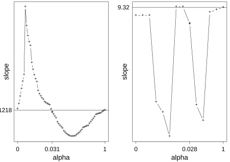
0 < α_b∗ < 1, should satisfy bγ(αb∗) ≈ bγ(1). Plots of bγ(α) versus α are informative and should be

examined in particular applications. They sometimes reveal a clear, well-defined value of αb∗; and

in cases where they do not, the ambiguity usually is a consequence of two or more nearly identically

good models corresponding to two or more close values of α. In practice all such models should

be considered. However, for our Monte Carlo study it was necessary to implement an automated

method of identifying a particular αb∗ and the corresponding model. We define αb∗ as the smallest

value of α that is greater than α_b0, where

b

α0 = Max{α <1 :bγ(α)>bγ(1) orbγ(α) is a local maximum} (9)

The defining rule is illustrated in Figure 3, where the models selected are marked by L

.

A key to our tuning procedure is that after white noise is added to the original data, forward

selection should yield a different sequence of candidate models, which helps distinguish the optimal

value of α. We need to add enough noise in order to introduce sufficient variation among the

sequences. But the noise level should not be too high, otherwise MSE(λ, α) is not (approximately)

linear in λ. In a pilot study, we set λ = (0.25,0.5,0.75,1,1.5,2,3,4) and fitted the simple linear

regression of MSE(λ, α) on different combinations of the aboveλ’s and found thatλ= (0.5,1,1.5,2)

provides satisfactory results. Note that the MSE from the original data (corresponding to λ= 0),

is not included in the simple linear regression to estimate the slope. This is because there is no

Monte Carlo variation at λ= 0 to smooth out discontinuities in MSE(0, α) as a function of α.

(15)

+ +

+ ++

+

++++ +

+

+ +

+ +₊

+ +

+

++_+++++++++++++++ ++++

+++++++++ +++++

+++++++ ++++

++++++ ++++++

++

O

0 0.028

alpha

1

(a)

slope

1.110

+ +

+++ +

+++++₊

+

+ +

+ ++₊₊

+++++++++++++++++++ +++

+++ ++++

++++++ ++

++ +++

++++

++++++++++ ++

O

0 0.034

alpha

1

(b)

slope

1.245

Figure 3: Demonstration of the Tuning Procedure

(a): α_b_∗ identified by a crossing of the baseline

(16)

slopes. The pilot study also suggested that the grid of α values is important. The finer the grid

the better, but this increases the computational burden. We found that no universal set works

for all data sets, and we suggest choosing the α’s adaptively based on the real data under study.

For a given real data set, the order of the predictors entering the model in forward selection is

determined, and so is the significance level associated with each step (more than one predictor can

enter the model at one step). Suppose the full model is obtained after k steps (k _≤ pmax), and

the associated significance levels are 0 < a1 < a2 < . . . < ak < 1. Then we chose the α’s as 0,

{ai+5ai

−1

6 ,

2ai+4ai

−1

6 ,

3ai+3ai

−1

6 ,

4ai+2ai

−1

6 ,

5ai+ai

−1

6 , i= 1,2, . . . , k}, 1+2ak

3 , 2+ak

3 , and 1, where a0 = 0.

4. MONTE CARLO STUDY

We performed a simulation study designed to compare our proposed method (hereafter called

NAMS, which stands for Noise Addition Model Selection), to ICp/F R, LB, and Minimum Cp.

Minimum Cp is based on all subsets, and ICp/F R and LB are based on forward selection

candi-date models. In addition, the model with the minimum model error among the forward selection

candidate models was identified and designated “Best” (which is the best that a forward selection

procedure can do in prediction, though in practice we do not have such information).

4.1 Simulation Setup

The setup of the simulation follows closely, and extends somewhat, the setup in Tibshirani and

Knight (1999), which is a simplified version of Breiman (1992). In the base simulation each data

set contains 21 predictors with n = 50 or 150 observations. The predictors follow a multivariate

normal distribution with mean 0 and covariance between xi and xj equal to ρ|i−j|, withρ= 0, 0.3,

and 0.7, respectively. The design matrices are fixed once generated. We have six different design

(17)

(those with non-zero coefficient) are generated in two clusters, around x7 and x14. Their initial

values are

β7+j = (h−j)2, |j|< h

β14+j = (h−j)2, |j|< h

(10)

The values h = 1,2,3,4 are used, resulting in 2,6,10 and 14 non-zero coefficients, respectively.

In addition, the null model H0 (all the coefficients are 0) and the full model FULL (with the

coefficients generated randomly from Uniform(0.5,1.5)) are also included. The regression equation

error follows a standard normal distribution. Except for H0, the coefficients of each model are

multiplied by a common constant so as to make the theoretical R2

equal to 0.75. Theoretical R2

is

defined as

TheoreticalR2

= (µ−µ01)

T ₍_µ₋_µ₀₁₎

(µ₋µ01)T ₍_µ₋_µ₀₁_{) +}_{n σ}2, (11)

where σ2

is the error variance,1 is a vector of 1’s, andµ0 =µT 1/n.

For a given combination ofnand ρ, we generate 100 data sets independently based on the same

design matrix and coefficients. All five variable selection methods are applied to each data set. The

true model is fit as well. For each method, the mean is calculated for both the model size and the

model error.

We augmented the base simulation study with three additional cases. In the first we took

n = 150 with 42 predictors (the original 21 predictors and their squares), in order to study how

the different methods perform in the presence of additional unimportant variables. In the second

we set n = 500 with the original 21 predictors, in order to study the performance of the methods

with a larger sample size. In the third, we reran the simulations with n = 150 observations and

21 predictors adjusting the coefficients so that the theoretical R2

equaled 0.35, 0.95 and 0.99,

respectively. The third case allowed us to study the consistency of the methods as R2

(18)

1.

4.2 Simulation Results

For the simulations with 21 predictors (n = 150,50) and R2

= 0.75, the ratios of model error of

Best to model error of NAMS, ICp/F R, Minimum Cp and LB are calculated for each combination

ofn andρ, and plotted in Figure 4. The larger the ratio, the better the performance. Note that the

relative standard error of the estimates (standard error divided by estimate) in Figure 4 is about

0.23 for H0, 0.12 for H1, and 0.06 for H2-H4 and FULL, respectively. Similar relative standard

errors are found in the other figures. We did not see much difference between the simulation result

with 150 observations and that with 50 observations, except that all the methods have poorer

performance when the sample size is smaller. Therefore, we concentrate on the simulation result

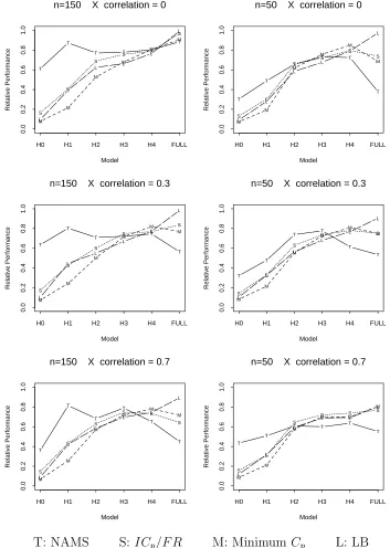
with 150 observations. Figure 4 shows that NAMS is the best in terms of model error when the true

model is H0, H1, H2, or H3. For FULL, NAMS loses to all the other methods. For H4, NAMS is

still the best when the predictors are uncorrelated, but as the correlation increases, NAMS underfits

and loses to the other methods. In addition, NAMS is the most stable in relative performance with

respect to Best, as indicated by its relatively flat performance curve. ICp/F R, Minimum Cp and

LB provide better relative performance as the true model increases in size; however, they do so at

the expense of overfitting models of small and moderate sizes. This claim is supported by Figure 5,

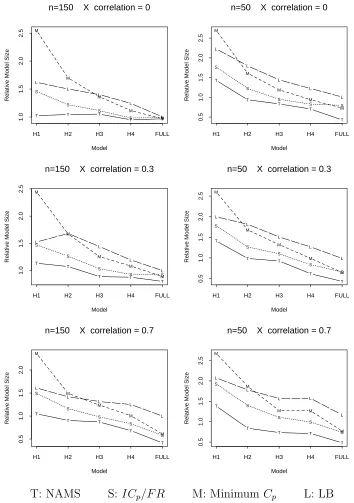
where the ratios of model size of NAMS, ICp/F R, Minimum Cp and LB to model size of True

are plotted for each combination of n and ρ. Figure 5 shows that NAMS always selects the most

parsimonious models, while LB and Minimum Cp select much larger models especially for H0-H2.

Therefore, NAMS is the best in achieving dimension reduction.

For the simulation with 42 predictors, 150 observations, and R2

= 0.75, the ratios of model

(19)

Model

Relative Performance

H0 H1 H2 H3 H4 FULL

0.0 0.2 0.4 0.6 0.8 1.0 T T

T T T

T S S S S S S M M M M M M L L L L L L

n=150 X correlation = 0

Model

H0 H1 H2 H3 H4 FULL

0.0 0.2 0.4 0.6 0.8 1.0 T T T T T T S S S S S S M M M M M M L L L L L L

Model

H0 H1 H2 H3 H4 FULL

0.0 0.2 0.4 0.6 0.8 1.0 T T

T T T

T S S S S S S M M M M M M L L L L L L

n=150 X correlation = 0.3

Model

H0 H1 H2 H3 H4 FULL

0.0 0.2 0.4 0.6 0.8 1.0 T T T T T T S S S

S S S

M M M M M M L L L L L L

Model

H0 H1 H2 H3 H4 FULL

0.0 0.2 0.4 0.6 0.8 1.0 T T T T T T S S S S S S M M M M M M L L L L L L

Model

H0 H1 H2 H3 H4 FULL

0.0 0.2 0.4 0.6 0.8 1.0 T T

T T T

T

S S

S

S S S

M M M M M M L L L L L L

T: NAMS S:ICp/F R M: Minimum Cp L: LB

Figure 4: Relative Performance with Respect to Best (21 predictors).

(20)

Model

Relative Model Size

H1 H2 H3 H4 FULL

1.0

1.5

2.0

2.5

T T T

T T

S S

S

S S

M

M M L

L L

Model

Relative Model Size

H1 H2 H3 H4 FULL

0.5

1.0

1.5

2.0

2.5

T

T T

T T S

S S

M

M M

M L

L

L L

L

Model

Relative Model Size

H1 H2 H3 H4 FULL

1.0

1.5

2.0

2.5

T T

T S

S S

M

M M

M L

L L

Model

Relative Model Size

H1 H2 H3 H4 FULL

0.5

1.0

1.5

2.0

2.5

T

T T

T T S

S S

S S M

M

M M

M L

L L

Model

Relative Model Size

H1 H2 H3 H4 FULL

0.5

1.0

1.5

2.0

T

T _T

T T S

S S

S S M

M M

M

M L

L L

Model

Relative Model Size

H1 H2 H3 H4 FULL

0.5

1.0

1.5

2.0

2.5

T

T T

T S

S S

S S M

M

M M

M L

L

L L

L

Figure 5: Relative Model Size with Respect to Best (21 predictors).

(21)

for each ρ. NAMS has the smallest model error for H0-H4 regardless of ρ, and for FULL when

ρ = 0, 0.3. Moreover, NAMS does not lose as much to the other methods as in the simulation

with 21 predictors on FULL with ρ = 0.7. The other three methods are adversely affected by the

additional 21 predictors, and their model errors increase substantially as the number of predictors

increases from 21 to 42. However, NAMS is less affected by the additional predictors and its model

error does not increase as much as the number of predictors increases from 21 (Figure 4) to 42

(Figure 6). It is evident in Figure 6 that NAMS is the overall method of choice forn = 150 and 42

predictors.

Figure 7 displays results from the simulation with n = 500 observations, R2

= 0.75 and the

original 21 predictors. All methods have much smaller model errors compared to the simulation

results with 150 observations, and they are closer to True and Best. Because overfitting is not

penalized as much when the sample size is large, NAMS does not outperform the other three

methods as much on H0-H3. However, for H4 and FULL, NAMS is nearly as good as the others,

except for FULL with ρ= 0.7.

Finally, the simulation with differentR2

showed that as R2

approaches 1, the model error of all

methods approached 0. This experiment, whose results are not displayed in this paper, used the

same design matrix and error for all R2

. We adjusted the coefficients instead of the error variance,

to get the desired theoretical R2

.

4.3 Conclusion and Discussion

From the simulation with 150 observations and 21 predictors (Figures 4, 5), we see that in terms

of model error, NAMS is the best when the true model is simple (H0-H2). It is marginally better

than the other methods when the true model is H3. It provides the best prediction by using

(22)

Model

H0 H1 H2 H3 H4 FULL

0.0

0.2

0.4

0.6

0.8

1.0

T

T T

T

S

M

L

L L

L

Model

H0 H1 H2 H3 H4 FULL

0.0

0.2

0.4

0.6

0.8

1.0

T

T _T

T

T T

S

M

M M

M

L

Model

H0 H1 H2 H3 H4 FULL

0.0

0.2

0.4

0.6

0.8

1.0

T

S

S S

M

L

L L

L

Figure 6: Relative Performance with Respect to Best (150 observations and 42 predictors).

(23)

Model

H0 H1 H2 H3 H4 FULL

0.0

0.2

0.4

0.6

0.8

1.0

T

T T

T

S

M

L

Model

H0 H1 H2 H3 H4 FULL

0.0

0.2

0.4

0.6

0.8

1.0

T

T T

T

S

M

L

Model

H0 H1 H2 H3 H4 FULL

0.0

0.2

0.4

0.6

0.8

1.0

T

T T

T

S

M

L

Figure 7: Relative Performance with Respect to Best (500 observations and 21 predictors).

(24)

others if the true model is complicated (H4 or FULL), especially when the correlation between the

predictors is high. But as shown in Figure 4, NAMS is the most stable in relative performance with

respect to Best, while ICp/F R, Minimum Cp and LB tend to overfit. Because they overfit, these

three methods provide better relative performance as the model gets more complicated. On the

whole, Minimum Cp overfits badly and provides very poor performance and is not recommended in

practice. ICp/F R is better than Minimum Cp except for H4.

We see a similar pattern in the simulation with 50 observations and 21 predictors, except that

every method performs worse due to the small sample size. When the sample size is 50, the ratio

of the number of predictors to the number of observations is greater than 0.25 so that it is difficult

to find a satisfactory model (Freedman et al. 1992).

For 500 observations and 21 predictors (Figure 7), all of the methods perform better, especially

for H4 and FULL, and all have similar model errors in most cases. However, Minimum Cp overfits

badly for H0-H2. NAMS has the smallest model error for H0-H2. There is not much difference

between the four methods for H3, H4 and FULL, except that NAMS loses to the other methods for

FULL with ρ = 0.7. We also recorded average mean squared errors (MSE) of the models selected

by the different methods. With the exception of FULL, ICp/F R, Minimum Cp and LB always

had Average MSE <1 (= the true error variance), indicating that these methods tended to overfit

thereby underestimating residual variation. NAMS unbiasedly estimated error variance in all cases

except for FULL.

The simulation with 150 observations and 42 predictors (Figure 6) shows that NAMS successfully

ignores the additional unimportant variables and outperforms the other methods except for the

FULL model when ρ = 0.7. The other three methods frequently fit the unimportant variables,

(25)

NAMS has the best prediction ability when the true model is simple. For complicated models

with greater correlation in the design matrix, NAMS loses to the other three methods in terms

of model error due to its tendency to underfit; but NAMS is as good as or better than the other

methods if either the sample size or the theoretical R2

is large. In addition, NAMS provides much

better performance than any of the other three methods when the number of predictors is large,

except for FULL with ρ = 0.7. In summary, NAMS is good at finding a parsimonious model

without sacrificing prediction ability when such a model exists.

5. EXAMPLES

We now illustrate the method on two data sets.

Pollution Data. (McDonald and Schwing 1973). This data set has 60 observations and 15

predictors. The response variable is the Total Age Adjusted Mortality Rate obtained for the

years 1959₋1961 for 201 Standard Metropolitan Statistical Areas (SMSA). The result from ridge

regression is copied from McDonald and Schwing (1973). We apply NAMS, LB,ICp/F R, Minimum

Cp, and Intelligent Cp to the data. The results are summarized in Table 1. All the methods have

similar performance in terms of model size and R2

. NAMS, ICp/F R and ICp select the same

five-variable model. LB and Minimum Cp select the same variable model, and a different

six-variable model was chosen by McDonald and Schwing (1973) using ridge regression. For NAMS,

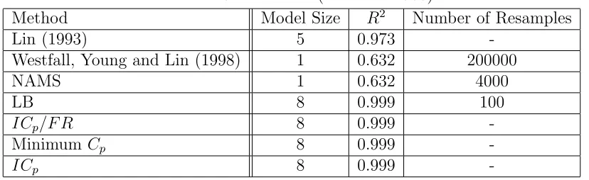
α0 is estimated to be 0.03 which corresponds to a five-variable model (1, 2, 6, 9, 14). Figure 8 (left

panel) displays the slope-versus-α plot from which the optimal choice of α was obtained.

Rubber Data. (Lin 1993). The original data set in Williams (1968) contains 28 runs and 23

predictors (there were 24 predictors in the paper, but two of them are identical). Lin (1993)

took half of the data set (14 runs and 23 predictors) to demonstrate the use of supersaturated

(26)

Table 1: Pollution Data

Method Variables Selected Model Size R2

Number of Resamples

Ridge Regression∗ 1,2,6,8,9,14 6 0.724

-NAMS 1,2,6,9,14 5 0.717 4000

LB 1,2,3,6,9,14 6 0.735 100

ICp/F R 1,2,6,9,14 5 0.717

-Minimum Cp 1,2,3,6,9,14 6 0.735

-ICp 1,2,6,9,14 5 0.717

-∗ _{From McDonald and Schwing (1973)}

Table 2: Rubber Data (Williams 1968)

Method Model Size R2

Number of Resamples

Lin (1993) 5 0.973

-Westfall, Young and Lin (1998) 1 0.632 200000

NAMS 1 0.632 4000

LB 8 0.999 100

ICp/F R 8 0.999

-Minimum Cp 8 0.999

-ICp 8 0.999

-to analyze the data and “the important fac-tors were identified as 15, 12, 20, 4, and 10 with an

R2

= 97.3%.” As pointed out by Wang (1995), factors 10 and 15 do not show up even in a model

with R2

= 0.99 when forward selection is applied to the other half of the data set. Later, Westfall,

Young and Lin (1998) attributed this inconsistency to multiple testing and developed a

resampling-based method to adjust the p-value for multiplicity. As shown in their Table 3, only one variable

(factor 15; adjusted p-value 0.016) is selected, because the next candidate variable, factor 12, has

an adjusted p-value of 0.816, and is deemed as non-significant.

The mean squared error from the full model provides the reference line used by the NAMS

method to tune forward selection. Thus NAMS is not directly applicable to super saturated designs

(SSD). However, such designs are commonly used under the assumption ofeffect sparsity, i.e., when

only a few of the many predictors are thought to be important. In such cases a liberal, initial model

fit resulting in a highR2

(27)

+ +

+

+ +

+

+ +

++₊ +++++

+ +

+ ++

++ +++

+++_++++++++++++ +++++

++++ ++++++

+++

o

0 0.031 1

1218

alpha

slope

+ + +

+

+ + +

+

+ + +

+

o

0 0.028 1

9.32

alpha

slope

Figure 8: Slope-versus-alpha plots for the real data examples. Circled point L

indicates optimal α.

Left panel, Pollution data; right panel, Rubber data.

adaptation of NAMS for SSDs. In the first stage use a liberal model fitting strategy to obtain a

collection of predictors resulting in a large R2

. Then starting with the predictors so identified, use

NAMS to pare down the set of predictors. We now show that this two-stage approach produces a

reasonable model for the Rubber data.

In the Rubber data, the model with 8 predictors from forward selection has an R2

= 1.000.

So, we concentrate on these 8 predictors. NAMS, LB, ICp/F R, Minimum Cp and Intelligent Cp

were applied to select models. As shown in Table 2, NAMS selects the one-variable model with α0

estimated to be 0.028, while LB, MinimumCp,ICp, andICp/F Rall select an eight-variable model,

(28)

We also applied the five methods using pilot studies with the first 3, 4, 5, 6, and 7 predictors

selected in forward selection, respectively, and obtained very consistent results: NAMS always

selects the one-variable model, while the other methods always select the largest possible model.

As another way to evaluate the methods, we applied them to the original data set (28

obser-vations and 23 predictors). LB, ICp, and ICp/F R select a three-variable model, and Minimum

Cp selects a five-variable model (note that the predictors enter the model in a different order in

the original data). NAMS again selects the same one-variable model (factor 15), while the other

methods apparently overfit the data.

REFERENCES

Atkinson, A. C. (1980), “A Note on the Generalized Information Criterion for Choice of a

Model,” Biometrika, 67, 413–418.

Breiman, L. (1992), “The Little Bootstrap and Other Methods for Dimensionality Selection in

Regression: X-Fixed Prediction Error,” J. Am. Stat. Assoc., 87, 738–754.

Carroll, R. J., Ruppert, D. and Stefanski, L. A. (1995),Measurement Error in Nonlinear Models,

London: Chapman Hall.

Cook, J. R. and Stefanski, L. A. (1994), “Simulation-Extrapolation Estimation in Parametric

Measurement Error Models,”J. Am. Stat. Assoc., 89, 1314–1328.

Draper, Norman R. and Smith, Harry (1981), Applied Regression Analysis (Second Edition),

New York: John Wiley & Sons.

Freedman, L. S., Pee, D., and Midthune, D. N. (1992), “The Problem of Underestimating the

Residual Error Variance in Forward Stepwise Regression,” Statistician, 41, 405–412.

(29)

Mallows, C. L. (1973), “Some Comments on Cp,”Technometrics, 15, 661–675.

Mallows, C. L. (1995), “More Comments onCp,” Technometrics, 37, 362–372.

McDonald, G. C. and Schwing, R. C. (1973), “Instabilities of Regression Estimates Relating

Air Pollution to Mortality,” Technometrics, 15, 463–481.

Shen, X. and Ye, J. (2002), “Adaptive Model Selection,” Journal of the American Statistical

Association 97, 210–221.

Stefanski, L. A. and Cook, J. R. (1995), “Simulation-Extrapolation: The Measurement Error

Jackknife,” Journal of the American Statistical Association 90, 1247–1256.

Tibshirani, R. and Knight, K. (1999), “The Covariance Inflation Criterion for Adaptive Model

Selection,” J. R. Statist. Soc., 61, 529–546.

Wang, P. C. (1995), “Letters to the Editor: Comments on Lin (1993),” Technometrics, 37,

358–359.

Westfall, P. H., Young, S. S. and Lin, D. K. J (1998), “Forward Selection Error Control in the

Analysis of Supersaturated Designs,” Statistica Sinica, 8, 101–117.

Williams, K. R. (1968), “Designed Experiments,”Rubber Age, 100, 65–71.

Ye, J. (1998), “On Measuring and Correcting the Effects of Data Mining and Model Selection,”

J. Am. Stat. Assoc., 93, 120–131.

Zhang, P. (1992), “On the Distributional Properties of Model Selection Criteria,” J. Am. Stat.