Effect of Rotation and Initial Stress on Generalized Thermoelastic Medium with Two-Temperature under Three-Phase-Lag Model

Effect of Rotation and Initial Stress on

Generalized Thermoelastic Medium with

Two-Temperature under Three-Phase-Lag Model

Mohamed I. A. Othman1, W. M. Hasona2_{, Nehal T. Mansour} 3

Department of Mathematics, Faculty of Science, Taif University 888, Saudi Arabia1

Department of Mathematics, Faculty of Science, Zagazig University, P.O. Box 44519, Zagazig, Egypt1,2,3

ABSTRACT:Three-phase-lag theory of thermoelasticity is employed to study the deformation of thermoelastic solid half-space under hydrostatic initial stress and rotation with two- temperature. The normal mode analysis is used to obtain the analytical expressions of the displacement components, force stress, thermodynamic temperature and conductive temperature. The numerical results are given and presented graphically when mechanical and thermal force is applied. Comparisons are made with the results predicted by three phase lag, Green-Naghdi III and Lord-Shulman in the presence and absence of initial stress as well as rotation.

KEYWORDS: Hydrostatic initial stress, Three-phase-lag, Thermoelastic, Thermodynamic temperature, Conductive temperature, Normal-mode.

I. INTRODUCTION

The generalized theory of thermoelasticity is one of the modified versions of classical uncoupled and coupled theory of thermoelasticity and has been developed in order to remove the paradox of physical impossible phenomena of infinite velocity of thermal signals in the classical coupled thermoelasticity. Five generalizations of the coupled theory of thermoelasticity have investigated [1]. The first generalization formulates the generalized thermoelasticity theory involving one thermal relaxation time [2]. The temperature rate-dependent thermo-elasticity is developed where includes two thermal relaxation times and does not violate the classical Fourier’s law of heat conduction, when the body under consideration has a center of symmetry [3]. One can review and presentation of generalized theories of thermoelasticity [4]. The wave propagation in anisotropic solids in generalized theories of thermoelasticity has studied [5-7]. The third generalization of the coupled theory of thermoelasticity is developed by Hetnarski and Ignaczak and is known as low-temperature thermoelasticity. The fourth generalization to the coupled theory of thermoelasticity introduced by Green and Naghdi and this theory is concerned with the thermoelasticity theory without energy dissipation, referred to as G-N theory of type II in which the classical Fourier law is replaced by a heat flux rate-temperature gradient relation and Green and Naghdi with energy dissipation referred to as G-N theory of type III. The fifth generalization of the coupled theory of thermoelasticity is referred to the dual-phase-lag thermoelasticity [8, 9]. Recently the three-phase-lag, heat conduction equation in which the Fourier law of heat conduction is replaced by an approximation to a modification of the Fourier law with the introduction of three different phases-lags for the heat flux vector, the temperature gradient and the thermal displacement gradient [10]. The stability of the three-phase-lag, the heat conduction equation is discussed [11]. Subsequently, this theory has employed of thermoelasticity with three-phase-lag to discuss a problem of thermoelastic interactions on functional graded orthotropic hollow sphere under thermal shock [12].

conducting elastic half-space was presented [14]. The effect of rotation on elastic waves has been studied [15, 16]. The effect of rotation in a magneto-thermoelastic medium was discussed [17].

The two-temperature theory of thermoelasticity was introduced [18-20], in which the classical Clausius-Duhem inequality was replaced by another one depending on two-temperature; the conductive temperature and the thermodynamic temperature, the first is due to the thermal processes, and the second is due to the mechanical processes inherent between the particles and the layers of elastic material, this theory was also investigated [21]. The two-temperature model was underrated and unnoticed for many years thereafter. Only in the last decade the theory has been noticed, developed in many works, and find its applications, mainly in the problems in which the discontinuities of stresses have no physical interpretations. Among the authors who contribute to developing this theory, it has studied existence, structural stability, convergence and spatial behavior of this theory [22], it was introduced the generalized Fourier law to the field equations of the two-temperature theory of thermoelasticity and proved the uniqueness of the solution for homogeneous isotropic material [23], the propagation of harmonic plane waves studied [24]. Recently, authors have studied the uniqueness and growth solutions [25], for the model proposed [23]. The effect of three-phase-lag on a two-temperature generalized thermoelasticity for the infinite medium with a spherical cavity had studied [26]. The initial stress present in the medium also has a considerable effect on the propagation of waves (Biot, 1965). Initial stress in solids has the significant influence on the mechanical response of the material from an initially stressed configuration and has applications in geophysics, engineering structures, and in the behavior of soft biological tissues. Initial stress arises from processes, such as manufacturing or growth and is present in the absence of applied loads. It has studied the effect of hydrostatic initial stress and rotation with Green-Naghdi (type III)thermoelastic half space with two-temperature [27]. It has studied the effect of initial stress on a generalized thermoelastic medium with the three-phase-lag model under temperature-dependent properties [28]. Effect of rotation and initial stress on an infinite generalized magneto-thermoelastic diffusing body with a spherical cavity had investigated [29]. Hall effects on unsteady flow due to no coaxial rotating disk and a fluid at infinity were studied [30]. Flow induced by non-coaxial rotation of a porous disk executing non-torsion oscillating and second grade fluid rotating at infinity was discussed [31].

The present paper is concerned with the investigations related to the effect of rotation and initial stress with two-temperature on a generalized thermoelastic medium based on the three-phase-lag model by applying the normal mode analysis. Also, the effects of rotation and initial stress on the physical quantities are discussed numerically and illustrated graphically.

Nomenclature

,

  Lame’s parameter counterparts

ui displacement vector

T thermodynamic temperature p initial stress

b constant material "two temperature parameter "

ρ

mass density

e

c

specific heat at constant strain K (≥0) thermal conductivity *

K _{material characteristic of the theory} δ_ij

Kronecker delta

v

τ phase lag of thermal displacement gradient

 conductive temperature

t τ

phase lag of temperature gradient τq phase lag of heat flux

ij

ω skew symmetric tensor called the rotation tensor

II. FORMULATION OF THE PROBLEM

We consider a homogeneous thermoelastic half-space with two-temperature rotating uniformly with angular velocity

Ω

additional terms [Schoenberg and Censor (1973)]: Centripetal acceleration Ω×(Ω× u)due to time varying motion only and Coriolis acceleration 2Ω× u _where u=(u , u ,1 2 0) is the dynamic displacement vector and angular velocity is Ω (0, 0,Ω). These terms, do not appear in non-rotating media.

III. BASIC EQUATIONS

The field equations and constitutive relations for a homogeneous isotropic thermoelastic solid with hydrostatic initial stress and rotation in the absence of incremental body forces and heat source are given by three phase lag model,

2 +

ij ij 0 ij ij ij

σ = μ e +[λ e γ T ( T )]δ p ω( δ ). (1)

The equation of motion

= + +

ij, j i i i

σ ρ u[ {Ω(Ωu)} (2Ωu) ]. (2)

The equation of heat conduction under three phase lag model 2 ₂

2 2 2

2

+ 1+ + +

2!

q

* *

v t q e 0

τ

K τ + Kτ τ ρc T γT e

t t

  

    = ( ∂ ∂ )(  ).

∂ ∂ (3)

Where, τv* (K + K τ* v),

2

= (1 ) ,

T b  (4)

1

= ( ),

2

ij i, j j,i

e u +u (5)

1

= ( ).

2

ij j,i i, j

ω u u (6)

For a two-dimensional problem in xy-plane, Eqs. (3.2) and (3.3) can be written as: 2

2 2 1 2 2

1 2

( ) + ( + + ) (1 ) [ 2 ],

2 1 2 x

u u

p p e

μ u λ μ γ b ρ u Ω Ω

x t t



 

 ∂   ∂ = ∂   ∂

∂ ∂ ∂ ∂ (7)

2

2 2 2 2 1

2 ₂ 2

( ) + ( + + ) (1 ) [ + 2 ],

2 2

u u

p p e

μ u λ μ γ b ρ u Ω Ω

y y t t



 

 ∂   ∂ = ∂  ∂

∂ ∂ ∂ ∂ (8)

2

2 2 2

2 2 2 2

2 2 2

+ + = (1+ + )[( (1 ) + ].

2!

q

* *

v t q e 0

τ e

K τ Kτ τ ρc b γT

t t t t t

 

  

  ∂  ∂ ∂ ∂   ∂

∂ ∂ ∂ ∂ ∂ (9)

For the purpose of numerical evaluation, we introduce dimensionless variables

1

( _i) = ( _i),

0

x , y ,u x, y,u

c ω

   (t ,τ ,τ ,τ_{v q t})= 1(t,τ ,τ ,τ_{v q t}),

ω

   

2

γ

T = T

λ + μ  , = 2 ij ij 1 σ σ , λ μ  + 2 P P = λ + μ  _, Ω=ωΩ , 2 γ = λ + μ

 , c =₀2 λ + μ2 ,

ρ 2

0 = e K . ρc c

ω

Using the above dimensionless quantities, Eqs. (7)-( 9) become 2

2 1 2 2

1 ₂ 1

+

( ) + ( + ) (1 ) = [ 2 ],

2 2 + 2 2

2 * u u

μ p λ μ p e

u b uΩ Ω

λ + μ λ μ x x t t

   ∂    ∂ ∂   ∂ ∂ ∂ ∂ ∂ (10) 2

2 2 2 1

2 ₂ 2

+

( ) + ( + ) (1 ) = [ 2 ],

2 2 + 2 2

2 * u u

μ p λ μ p e

u b u Ω Ω

λ + μ λ μ x x t t

   ∂    ∂   ∂ ∂ ∂ ∂ ∂ ∂ (11) 2 ₂

2 2 2 2

1 + 2 + = (1+ + ₂)[(1 ) + 3 ].

2!

q *

t q

τ

ε ε τ τ b ε e

t t

   

     ∂ ∂    

Where, 1 ₂ 0 = * e K ε

ρc c , ε = + ε τ2 1 1 v,





2 3= 2 0 e γ T ε

ρc λ + μ , = ₀2 2

* b

b .

c ω

We define displacement potentials q and  which relate to displacement components u₁and

u

₂as,

1

=

,x , y

u

q



ψ

,

u

₂

=

q

_{, y}

+

ψ

_,x

.

(13)

Using Eq. (13) in Eqs. (10)-(12), we obtain: 2

2 2 2

2

( Ω )] + 2q Ω ψ * =0

t

t b 

   

 ∂ ∂ 

[ (1 ) ,

∂

∂ (14)

2

2 2

1 ₂

+ [ ( )] 0,

2Ω q a Ω ψ =

t  t 

 ∂  ∂

∂ ∂ (15)

2 ₂

2 2 2 2 2

1 + 2 + = (1+ + ₂)[(1 ) + 3 ].

2!

q *

t q

τ

ε ε τ τ b ε q

t t

   

     ∂ ∂     

∂ ∂ (16)

IV. NORMAL MODE ANALYSIS

The solution of the considered physical variable can be decomposed in terms of normal mode as the following form *

1 2 1 2

[u , u , e,T, , q,ψ, σ_ij](x, y,t) = [u ,u ,e ,T* * * *, ,q ,ψ ,σ* * *_ij]( )exp(y ωt+ iax).

(17) Where,  is the complex time constant and a is the wave number in x-direction.

Using (17) in Eqs. (14)-(16), we obtain

2 2 *

1 2

(D A q) * + (b*D A ) +2Ωωψ =* 0, (18)

2

1 3

( Da A )ψ* 2Ωωq = ,* 0 (19)

2 * 2 2

4 5 6

(A D A ) A (D a q = .) * 0 (20) Where,

2 2 2

1= ( + ),

A a ω Ω 2= 1 2,

*

A b a A3(a a1 2+ω2Ω2),

2 2 2

4 ( +1 2 + ) + (1+ + ),

2

q *

t q

τ ω

A  ε ε ω τ ω b τ ω

2

2 2 2 2

5= ( 1+ 2 + ) (1+ )[1+ + ],

2!

q *

t q

τ

A a ε ε ω τ ω  a b τ ω ω

2

2 2

6= 3 [1+ + ].

2!

q q

τ

A ε ω τ ω ω

Eliminating *

 and * between Eqs. (4.18)-(4.20), we get

6 4 2 *

[D AD + BD E]{q*( ),y  ( ),y ψ*( )} = 0.y (21)

Where,

2

1 5 1 4 2 6 6 3 4 6

1 4 6

{ + + + } + ( + )

= ,

( + )

* *

*

a A A A A A b a A A A b A

A

a A A b

2 2 2 2

3 5 1 1 5 1 3 4 4 2 3 6 3 6 1 2 6

1 4 6

4

,

( )

*

*

A A + a A A + A A A + A Ω ω + A A A +b a A A + a a A A

B =

a A + A b

2 2 2

1 3 5 5 2 3 6

1 4 6

4

,

( *)

A A A + A Ω ω + a A A A

E =

a A + A b

D= d . dy

The solution of Eq. (21) which are bound as y , has the form 3 1 = y * _n n n= k

3

1

= k y

* _n

1n n n=

ψ

_

H M e , (23)

3 *

1

= k yn

2n n n=

H M e ,



_

 (24)

1 = 3 y * _n 3n n n= k

T

_

H M e . (25)

Where M_n(n1, 2,3)are some constants, k_n2 are the roots of the characteristic equation of Eq. (21). Dimensionless variables of the stress components as the following,

1 ₂ 2,

2 = + (1 )

xx ,x y

σ u u T P,

β

   (26)

2, 2 1

2

= + (1 )

yy y ,x

σ u u T P,

β

   (27)

2 1 1 2

= +

xy ,y ,x

σ a u a u , (28)

1 1 2

= +

yx ,y 2,x

σ a u a u . (29)

Using Eq. (13) and Eqs. (22)-(25) in (26)-(29) 3 1 4 1 ( + ) n n n=

ωt k_ny i a x

u =

_

H M e  , (30)

3 2 1 ( + ) , 5n n n

ωt k_ny i a x

u = H M e







(31)

3

1

( + )

, xx 6n n

n=

ωt k_ny i a x

σ =



H M e  P

(32)

3

7 1

( + )

= ,

yy n n

n =

ωt k_ny i a x

σ

_

H M e  P (33)

3

( + )

8 1

= ωt kny i a x ,

x y n n

n =

σ

_

H M e  (34)

3

( + )

9 1

= ωt kny i a x ,

yx n n

n =

σ

_

H M e  (35)

3

( + )

3 1

= ωt kny i a x .

n n n =

T

_

H M e  (36)

Where, 2 1 3 2 = , ( ) 1n n Ωω H

a k A

2 2 6 2 ₂ 4 5 ( ) = , ( ) n n n

k a A

H

A k A

 

2 2

3 = [1 ( )],

*

n 2n n

H H b k a H_4n = (ia+k H_{n 1n}), H_5n=(k_n+iaH_1n),

6 4 ₂ 5 3

2

[i (1 ) ],

n n n n n

H = aH k H H

β

   7 5 4 ₂ 3

2

= [ + (1 ) ],

n n n n n

H k H ia H H

β

   H_8n = (a k H_{2 n 4n} +iaa H_{2 5n}),

9n = ( 1 n 4n+ 2 5n),

H a k H i a a H ₁ 1₂

2

p

a = ,

β  2 2

1 = + 2 p a , β

2 + 2

=λ μ

β .

V. THE BOUNDARY CONDITIONS

The boundary conditions on the plane surface y 0 are:

( + )

1

+ ω t i a x

x x

σ =  P P e ,

( + )

2

ω t iax

T = P e ,

σxy = .0 (37)

Using Eqs. (32), (34) and (36) in boundary conditions (37), we get three equations in three constants M_n(n1, 2,3) as: 3

6 1

1

n n n=

H M = P ,



(38)

3 8 1

0

n n n=

H M = ,



(39)

3

3 2

1

n n n=

H M = P .



(40)

Solving Eqs. (38)-(40) the constants Mn (n1, 2,3)are defined as follows:

1 1 ,

Δ

M =

Δ

2 2

Δ

M =

Δ ,

3 3

Δ

M = .

Δ

Where, Δ = H61(H H82 33H H83 32)H62(H H81 33H H83 31)+ H63(H H81 32H H82 31),

1 1( 82 33 83 32) 2( 83 62 63 82),

Δ = P H H H H + P H H H H

Δ = P H H2  1( 81 33H H83 31)+ P H H2( 63 81H H61 83), 3 1( 81 32 82 31) 2( 61 82 62 81).

Δ = P H H H H + P H H H H

VI. NUMERICAL RESULTS

To study the effect of rotation and initial stress, we now present some numerical results. For this purpose, copper is taken as the thermoelastic material for which we take the following values of the different physical constants.

10 7.7 10

   2

.

N M  _,

10 1 2

3.86 10 . .

μ   Kg m s ,

K 300w m. 1.K1,

5 1

1.78 10 ,

t

α    K 8954Kg m. 3, 1 1

383.1 .

E

C  J KgK , T₀ 293K , a0.5, ω = ω + iξ₀ , ₀ 0.1, K*2.97 10 , 13 0.6,

x 0.5, 0.3,

t  p₁2, p₂3, b 0.1,

v= 0.05 , t= 0.2 , q= 0.8.

The numerical technique, outlined above, was used for the distribution of the real part of the temperature T, the displacement components u,v and the stress components x x,yy,xy for the problem. Here, all the variables are

taken in non-dimensional form the result. Fig. 1-6 show the distribution of the physical quantities based on L-S, G-N III and 3PHL in the case of p =0,1. Fig. 1 depicts that the displacement component u increases with the decrease of initial stress in the three theories. In the absence of initial stress (i.e. p = 0 ), u begins to increase then smooth decreases again to try to return to zero at infinity and in the presence of initial stress (i.e. p =1), u decreases and increases until it develops to zero.

Fig. 1Distribution of displacement component u in the absence and presence of p

0 2 4 6 8 10 12 14 16 18 20

-200 -150 -100 -50 0 50 100

y

u

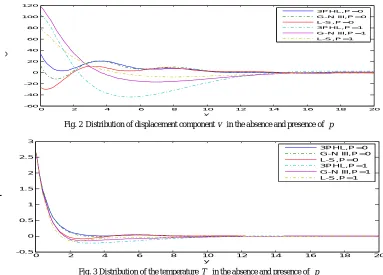
Fig. 2 exhibits that the displacement component

v

decreases with the decrease of initial stress and it is increasing with the increase of initial stress, based on L-S, G-N III and 3PHL, that’s means that the displacement v is directly proportional to initial stress, and take the form of a wave until it develops to zero.Fig. 3 demonstrates that the behavior of temperature T decays meaning that the temperature decrease for p =0,1 and take the form of a wave until it develops to zero.

Fig. 2Distribution of displacement component v in the absence and presence of p

Fig. 3Distribution of the temperature T in the absence and presence of p

Fig. 4 represents that the stress component xy increase with the increase of initial stress p in three theories and take

the form of the wave until it develops to zero, and decreasing with the decrease of the initial stress in three theories and take the form of the wave until it develops to zero.

Fig. 4Distribution of the stress component σx y in the absence and presence of p

Fig. 5 depicts that the stress component σ_{x x} begins from the value 2 and satisfies the boundary condition at y 0 in three theories. The stress component σx x increase with the decrease of initial stress and decays to zero. Fig. 6 explains

that the stress component yy increase with the decrease of initial stress and take the form of the wave until it

0 2 4 6 8 10 12 14 16 18 20

-60 -40 -20 0 20 40 60 80 100 120

y

v

3PHL,P= 0 G-N III, P= 0 L-S, P=0 3PHL,P= 1 G-N III, P= 1 L-S, P=1

0 2 4 6 8 10 12 14 16 18 20

-0.5 0 0.5 1 1.5 2 2.5 3

y

T

3PHL,P=0 G-N III,P=0 L-S,P= 0 3PHL,P=1 G-N III,P=1 L-S,P= 1

0 2 4 6 8 10 12 14 16 18 20

-20 0 20 40 60 80 100

y

 x

y

develops to zero. Figs. 7-12 exhibit the distribution of the physical quantities based on L-S, G-N III and 3PHL in the case of Ω =0, 0.2.

Fig. 5Distribution of the stress componentσx x in the absence and presence of p

Fig. 6Distribution of the stress componentσyy in the absence and presence of p

Fig. 7 shows that at Ω = 0,the stress component yy is decreasing to a minimum value in the range 0 y 2, while,

increases in the range 2 y 4 and decays to zero in L-S, G-N III and 3PHL theories, but at Ω = 0.2,it decreases to a minimum value in the range 0 y 1, and increases in the range 1 y 3, until it develops to zero.

Fig. 7Distribution of the stress component σyy in the absence and presence of rotation

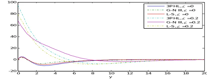
Fig. 8 shows that at Ω = 0, _{the stress component} σx x satisfies the boundary condition and decreasing to a minimum value in the range 0 y 1,while, increases in the range 1 y 6 and decays to zero in the context of three theories. However, at Ω = 0.2, _{it increases in the range} 0 y 2, then, decreases in the range 2 y 8 and decays to zero in the three theories.

0 2 4 6 8 10 12 14 16 18 20

-40 -30 -20 -10 0 10 20 30

y

 x

x

3P HL,P=0 G-N III,P=0 L-S ,P=0 3P HL,P=1 G-N III,P=1 L-S ,P=1

0 2 4 6 8 10 12 14 16 18 20

-60 -50 -40 -30 -20 -10 0 10 20 30

y

 y

y

3P HL,P =0 G-N III, P= 0 L-S, P=0 3P HL,P =1 G-N III, P= 1 L-S, P=1

0 2 4 6 8 10 12 14 16 18 20

-30 -20 -10 0 10 20 30

y

 y

y

Fig. 8 Distribution of the stress componentσx x in the absence and presence of rotation

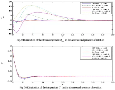
Fig. 9 explains that in the absence of rotation the stress component xy decreases in the range 0 y 1, in three

theories, and increases in the range 1y 3. While in the presence of rotation, xy decreases in the range 0 y 1,

then, increases in the range 2 y 5 and take the form of the wave until it develops to zero in L-S and G-N III and 3PHL theories.

Fig. 9Distribution of the stress component σx y in the absence and presence of rotation

Fig. 10Distribution of the temperature T in the absence and presence of rotation

Fig. 10 demonstrates that the temperature satisfies the boundary condition at y 0 and decreases, in the three theories at  0, 0.2, _{to a minimum value in the range} 0 y 2 and increasing in the range 2 y 4, until it decays to zero. Fig. 11shows that the displacement component v increases at Ω = 0.2, in three theories, and decreases at  0, that’s mean that the displacement component v increases with the increase of rotation and take the form of the wave

0 2 4 6 8 10 12 14 16 18 20

-20 -15 -10 -5 0 5 10 15

y

 x

x

3P HL,=0 G-N III,=0 L-S,= 0 3P HL,=0.2 G-N III,=0.2 L-S,= 0.2

0 2 4 6 8 10 12 14 16 18 20

-15 -10 -5 0 5 10 15 20

y

 x

y

3PHL,= 0 G-N III,= 0 L-S,= 0 3PHL,= 0. 2 G-N III,= 0.2 L-S,= 0. 2

0 2 4 6 8 10 12 14 16 18 20

-0.5 0 0.5 1 1.5 2 2.5 3

y

T

until it develops to zero.Fig. 12 depicts that the displacement component u increases with the decrease of rotation and try to return to zero at infinity.

Fig. 11Distribution of displacement component v in the absence and presence of rotation

Fig.12Distribution of displacement component u in the absence and presence of rotation

VII. CONCLUSION

The figures obtained by comparing the three theories, important phenomena are observed:

1. Analytical solutions based upon normal mode analysis of the thermoelastic problem in solids have been developed.

2. The method that is used in the present article is applicable to a wide range of problems in hydrodynamics and thermoelasticity.

3. There are significant differences in the field quantities under GN-III, 3PHL and L-S theories. 4. The presence of the initial stress and rotation plays a significant role in all physical quantities. 5. All the physical quantities satisfy the boundary conditions.

6. The comparison of different theories of thermoelasticity, i.e. L-S theory, the model of 3PL and the GN-III is carried out.

7. The value of all the physical quantities converges to zero, and all the functions are continuous.

REFERENCES

[1] Hetnarski, R.B. and Ignaczak, J. ''Generalized Thermoelasticity", Journal of Thermal stresses, vol 22, pp. 451-476, 1999.

[2] Lord, H.W. and Shulman, Y. "A generalized dynamical theory of thermoelasticity", Journal of the Mechanics and Physics of Solids, vol. 15, pp. 299-309, 1967.

[3] Green, A.E. and Lindsay K.A.''Thermoelasticity", Journal of Elasticity, vol. 2, pp. 1-7, 1972.

[4] Hetnarski, R.B. and Ignaczak, J. "Soliton-like waves in a low temperature non-linear thermoelastic solid", International journal of Engineering

0 2 4 6 8 10 12 14 16 18 20

-20 0 20 40 60 80 100

y

v

3PHL,=0 G-N III,=0 L-S,=0 3PHL,=0.2 G-N III,=0.2 L-S,=0.2

0 2 4 6 8 10 12 14 16 18 20

-50 -40 -30 -20 -10 0 10

y

u

Science, vol. 34, pp. 1767-1787, 1996.

[5] Sharma, J.N. and Sidhu, R.S. "On the Propagation of Plane harmonic waves in anisotropic generalized thermoelasticity", International Journal of Engineering Science, vol. 24, pp. 1511-1516, 1986.

[6] Singh, H. and Sharma, J.N."Generalized thermoelastic waves in transversely isotropic media", Journal of the Acoustical Society of America, vol.85, pp. 1407-1413, 1985.

[7] Singh, H. and Sharma, J.N. "Generalized thermoelastic waves in anisotropic media", Journal of the Acoustical Society of America, vol.77, pp. 1046-1053, 1985.

[8] Tzou, D.Y. "Aunified field approach for heat conduction from macro to micro scales", Asme journal of heat transfer, vol. 117, pp. 8-16, 1995. [9] Chandrasekharaiah, D.S. "Hyperbolic thermoelasticity: A review of recent Literature", Applied Mechanics Reviews, vol. 51, pp. 705-729,

1998.

[10] Roy Choudhuri, S. K. "On thermoelastic three phase lag model", Journal of Thermal Stresses, vol. 30, pp. 231-238, 2007.

[11] Quintanilla, R. and Racke, R. "A note on stability in three-phase-lag heat Conduction", International Journal of Heat and Mass Transfer, vol. 51, pp. 24-29, 2008.

[12] Kar, A. and Kanoria, M. "Generalized thermoelastic functionally graded orthotropic hollow sphere under thermal shock with three-phase-lag effect", European Journal of Mechanics - A/Solids, vol. 28, pp. 757-767, 2009.

[13] Schoenberg, M. and Censor D. "Elastic waves in rotating media", Quarterly Journal of Mechanics and Applied Mathematics, vol. 31, pp. 115-125, 1973.

[14] Chand, D. Sharma, J. N. and Sud, S. P. "Transient generalized magneto-thermoelastic waves in a rotating half space", International Journal of Engineering Science, vol. 28, pp. 547-556, 1990.

[15] Clarke, N. S. and Burdness, J. J. "Rayleigh waves on rotating surface", ASME Journal of Applied Mechanics. vol. 61, pp. 724-726, 1994. [16] Destrade, M. "Surface waves in rotating rhombic crystal", Proceeding of the royal society of London. Series A, vol. 460, pp. 653-665, 2004. [17] Othman, M. I. A. and Song, Y. Q. "The effect of rotation on 2-D thermal shock problems for a generalized magneto-thermoelasticity half

space under three theories", Mult. Model Math. & Structure, vol.5, pp. 43-58, 2009.

[18] Gurtin, M.E. and Williams, W.O. "An axiom foundation for continuum Thermodynamics", Archive for Rational Mechanics and Analysis, vol. 26, pp. 83-117, 1967.

[19] Chen, P.J. and Gurtin, M.E. "On a theory of heat conduction involving two temperatures", Zeitschrift für angewandte Mathematik und Physik, vol. 19, pp. 614-627, 1968.

[20] Chen, P.J. and Gurtin, M.E. "A note on non-simple heat Conduction, Z. Zeitschrift für angewandte Mathematik und Physik, vol. 19, pp. 969-970, 1968.

[21] Ieşan, D. "On the linear coupled thermoelasticity with two temperatures", Zeitschrift für angewandte Mathematik und Physik, vol, 21, pp. 583-591, 1970.

[22] Quintanilla, R. "On existence, structural stability, convergence and spatial behavior in thermoelasticity with two temperatures", Acta Mechanica, vol. 168, pp. 61–73, 2004.

[23] Youssef, H. M. "Theory of two-temperature generalized thermoelasticity", IMA journal of applied mathematics, vol. 71, pp. 383-390, 2006. [24] Puri, P. and Jordan, P. "On the propagation of harmonic plane waves under the two-temperature theory", International Journal of Engineering

Science, vol. 44, pp. 1113-1126, 2006.

[25] Magaña, A. and Quintanilla, R. "Uniqueness and growth of solutions in two-temperature generalized thermoelastic theories", Mathematics and Mechanics of Solids, vol. 14, pp. 622-634, 2009.

[26] Banik, S. and Kanoria, M. "Effects of three-phase-lag on two-temperature generalized thermoelasticity for infinite medium with spherical cavity", Journal of Applied Mathematics and Mechanics, vol. 33, pp. 483-498, 2011.

[27] Ailawalia, P. and Budhiraja, S. "On studied effect ofhydrostatic initial stress and rotation in Green-naghdi (type III)thermoelastic half space with two temperature, International Journal of Applied Mathematics and Mechanics, vol. 7, pp. 93-110, 2011.

[28] Othman, M. I. A , Hasona, W. M. and Eraki, E. E. M. "The effect of initial stress on generalized thermoelastic medium with three-phase-lag model under temperature-dependent properties" , Canadian Journal of physics, vol. 92, pp. 448-457, 2014.

[29] Abd-Alla, A.M. and Abo-Dahab, S.M. "effect of rotation and initial stress on an infinite generalized magneto-thermoelastic diffusion body with a spherical cavity", Journal of Thermal Stresses, vol. 35, pp. 892-912, 2012.

[30] Hayat, T. Ellahi, R. and Asghar, S. "Hall effects on unsteady flow due to non-coaxially rotating disk and a fluid at infinity", Chemical Engineering Communications, vol. 195, pp. 958-976, 2008.