Article
Low-Frequency Sea Surface Radar Doppler Echo
Yury Yu. Yurovsky1,2∗ ID, Vladimir N. Kudryavtsev1,2, Semyon A. Grodsky3and Bertrand Chapron2,4
1 Marine Hydrophysical Institute Russian Academy Sci., 2 Kapitanskaya, Sevastopol, Russia; [email protected]
2 Russian State Hydrometeorological University, 98 Malookhotinskiy, St-Petersburg, Russia; [email protected] 3 University of Maryland, College Park, MD, USA; [email protected]
4 Institut Français de Recherche pour l’Exploitation de la Mer, 29280, Plouzané, France;
1
2
3
4
5
6
7
8
9
10
* Correspondence:[email protected];Tel.:+7-978-789-11-31
Abstract: ObservedseasurfaceKa-bandnormalizedradarbackscattercrosssection(NRCS)and Dopplervelocity(DV)exhibitenergyatlowfrequencies(LF)belowthesurfacewaverange. Itis shownthatnon-linearityinNRCS-waveslopeModulationTransferFunction(MTF)andinherent NRCSaveragingwithinthefootprintaccountfortheNRCSandDVLFvariancewiththeexception ofVVNRCSforwhichalmosthalfoftheLFvarianceisattributabletowindfluctuations.Although thedistributionofradarDVisquasi-Gaussiansuggestingvirtuallylittleimpactofnon-linearity, theLFDVvariationsariseduetofootprintaveragingofcorrelatedlocalDVandnon-linearNRCS. NumericalsimulationsdemonstratethatMTFnon-linearityweaklyaffectstraditionallinearMTF estimate(lessthan10%for|MTF|<20).ThusthelinearMTFisagoodapproximationtoevaluate theDVaveragedoverlargefootprintstypicalofsatelliteobservations.
Keywords:Radar;ocean;backscatter;Dopplershift;wavegroups;non-linearity;modulation
11
1. Introduction 12
Doppler frequency shift of radar backscattering from the sea surface and corresponding Doppler
13
Velocity (DV) are governed by the surface kinematics. In early studies, the DV measured by a coherent
14
radar was used as a proxy for wave gauge (WG) to examine wave-induced modulations of the
15
normalized radar cross-section (NRCS) [1–3]. Further, along-track interferometry [4–6] as well as
16
Doppler centroid anomaly [7–9] methods were used to demonstrate an ability to detect surface currents
17
from air/space-borne radar platforms. Recently, the DV has been explored as a key parameter for
18
future satellite ocean current missions based on the Doppler rotating beam scatterometry [10–14].
19
Surface waves modulate local DV and NRCS and thus produce a wave-induced mean component
20
of the DV due to correlated modulations of DV and NRCS, which doesn’t zero after averaging over
21
long wave scales. The wave-induced DV is not small [6,9,15,16] and is important for retrieving surface
22
currents from measured DV.
23
Besides variation in the frequency range of surface waves, the DV and NRCS reveal a
24
low-frequency variation (LF) at sub-wave frequencies. Plant et al. [17] have found that LF NRCS
25
spectral density is comparable in size to wave-induced spectral density. It is larger for L-band than for
26
X-band and depends on wind. From these observations it has been concluded that LF NRCS variations
27
are not a system-related noise, but produced by turbulent wind fluctuations on sub-wave frequencies,
28
which are uncorrelated with surface waves. Alternatively, Grodsky et al. [18] have attributed LF NRCS
29
variations to wave groups (assuming constant wind).
30
The presence of X-band LF DV variations has been reported in [17,19]. Such variations are
31
especially large at HH polarization and increase with incidence angle (see Fig. 5 in [19]). Numerical
32
simulations of Plant [19] have shown that LF DV variations can be explained by fast scatterers
33
associated with the bound (parasitic) waves. Interestingly, at low grazing angles, Hwang et al. [20]
34
have found that radar-derived wave periods are longer by about 20–27% than those measured by
35
nearby buoy and explained this by wave breaking spikes present not on every dominant wave crest.
36
Given that breaking waves are related to wave groups [21], this mechanism is somewhat similar to
37
that proposed in [18].
38
If coherent for DV and NRCS [17], such LF variations may produce an additional time-mean
39
DV component after averaging over their time/space scales. Particularly, a real aperture Doppler
40
scatterometer with a few kilometer footprint inherently averages a product of LF DV and NRCS
41
variations. Besides wind-induced variations, the correlated LF variations of NRCS and DV may
42
originate from impacts of wave groups (via wave breaking and Stokes drift), oil slicks, Langmuir
43
circulations (via Bragg wave damping), small-scale current eddies, etc. Thus, the understanding of
44
nature of LF radar variations is important for accessing their impact on the time mean DV.
45
The origin of LF fluctuations is examined using Ka-band platform-based measurements [22,23]
46
that include well pronounced LF features. We focus on explanations of observed NRCS and DV spectra,
47
and their cross-spectrum, which define the time mean LF DV contribution. The analysis is based on
48
radar measurements and their comparison with concurrent wind and wave measurements. Using a
49
primitive numerical backscattering simulation, we demonstrate how the impact of LF variations can
50
be explained.
51
2. Experiment 52
The measurements were carried out in the Black sea from a static research platform located 600 m
53
offshore in a 30 m deep water. A Ka-band (37.5 GHz) dual-copolarized (VV and HH) continuous wave
54
Doppler radar was used to obtain time series of the sea surface NRCS and DV (details on the radar
55
calibration and measurement techniques are given in [22,23]). Simultaneous wave measurements were
56
performed using a resistant wire wave gauge (WG) operated at 20 Hz sampling rate. Wind velocity
57
was measured at 0.2 Hz sampling rate by a vane anemometer installed at 21 m height on platform
58
mast.
59
We select a typical one hour sample record that includes LF features. The radar was installed at
60
12 m height atθ=48◦incidence angle and directed upwind (wind and dominant waves both coming
61
from the east). For this observation geometry, the radar surface footprint was about 2 m in width and 4
62
m in length.
63
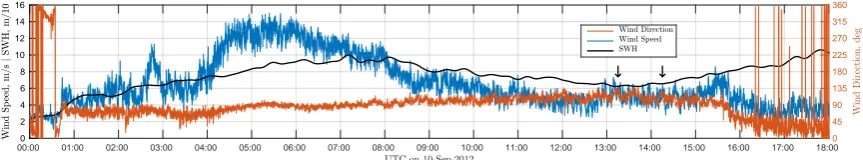
On the measurement day (12-Sep-2012, Fig.1), the wind speed accelerated at about 04:00 UTC
64
reaching maximum of about 15 m/s by 05:00 UTC. Wave development lagged the wind amplification
65
and then they calmed down after 18:00 UTC. The measurements, we consider, were taken between
66
13:20 UTC and 14:20 UTC when wind waves became steady and no strong swell present. During the
67
acquisition period, the mean wind speed was 6 m/s with 0.7 m significant wave height. The wind
68
wave spectrum (see Fig.3a below) was close to the saturation level for wave frequency>0.38 Hz (to
69
within the Toba empirical confidence range [24]) but had somewhat weaker spectral level between
70
0.19 Hz and 0.38 Hz. Based on the WG measurements, no surface waves were present below the
71
peak frequency, fp=0.19 Hz. Besides somewhat weaker peak spectrum level, the wave state can be 72
considered as a well developed forU=6 m/s (wave ageU/cp≈0.83). 73
3. Analyzed Parameters and their Relations 74
The instantaneous NRCS,σ(t), and DV,v(t), were computed as the 0th and 1st moments of
75
the instantaneous spectrum,S(f,t) =<|FFT(I+iQ)|2>, estimated using Fourier transform of raw 76
in-phase and quadrature signals, I/Q, see e.g., [20,25,26] over consecutiveτ =0.2-s time intervals,
77
[t−τ/2;t+τ/2],
78
σ(t) =
Z
S(f,t)df, (1)
v(t) = πkr−1 Z
00:00 01:00 02:00 03:00 04:00 05:00 06:00 07:00 08:00 09:00 10:00 11:00 12:00 13:00 14:00 15:00 16:00 17:00 18:00
0 2 4 6 8 10 12 14 16
0 45 90 135 180 225 270 315 360
Figure 1. Wind speed, wind direction, and significant wave height (SWH) on 12-Sep-2012. Radar
acquisition time span is marked by the two black arrows.
wherekr =785 rad/m is the radar wavenumber. 79
LF variations are visualized by applying the running time mean:
avg(X(t)) =
Z
X(t0)W(t0−t,∆)dt0, (3)
whereW(t,∆)is the normalized rectangular window with width,∆.
80
Signal envelope, reflecting group structure, is estimated using the running variance:
var(X(t)) =avg([X(t)−avg(X(t))]2) (4) The standard relationship between radar signal variations and wave parameters is employed [1,3]. Fourier harmonic of DV variations due to orbital velocities of resolved surface waves reads:
v=aωG, (5)
wherea= a(ω)is the Fourier harmonic of wave elevation,ωis the wave angular frequency,G =
cosφsinθ+icosθis the geometric coefficient accounting for horizontal and vertical orbital velocity
components,φis the azimuthal angle between wave vector and radar incidence plane,θis the incidence
angle. Thus, the Doppler velocity spectrumSvv, and the sea surface elevation spectrum,Szz, are related as
Szz=ω2|G|2Svv. (6)
whereSxystands for the cross-spectrum ofxandy. 81
In terms of linear Modulation Transfer Function (MTF), NRCS variation is a linear function of
82
wave slope [1,3]. For upwind radar measurements analyzed in this paper we suppose all waves are
83
traveling towards the radar (a unidirectional sea). The NRCS can then be expressed via mean and
84
variations:
85
σ=σ+σ0=σ(1+Mζ), (7)
whereσis the mean NRCS not disturbed by waves,σ0 = σ0(ω)is the Fourier harmonic of NRCS
86
variation,ζ=ζ(ω)is the Fourier harmonic of wave slope with amplitudeak,kis the wavenumber
87
corresponding toω, andM= M(ω)is the linear MTF.
88
The MTF can be evaluated from either WG or DV using the deep water gravity wave dispersion relationship,ω=pgk, (applicable to our measurements):
M= σ
0
σζ =
gSzσ
σω2Szz
= gGSvσ
σωSvv, (8) wheregis the gravity acceleration.
89
Conversely, if the MTF is known, the NRCS time series can be reconstructed from either WG or
90
-0.2 0 0.2 0.4 0.6 0.8 1 1.2 1.4
0 1 2 3 4 5 6 7
( a)
1000 1200 1400 1600 1800 2000 2200 2400 2600 2800 3000
-40 -35 -30 -25 -20 -15 -10 -5
0 1 2 3 4 5 6 7
( b )
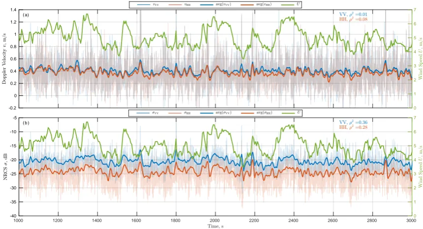
Figure 2.Time series of 10 s average (top panel) DV and (bottom panel) NRCS. Green – wind speed,
bold blue/orange – VV/HH,ρ2is the corresponding squared correlation wind wind speed.
the average magnitude of linear MTF is 13.5 and 17 for VV and HH polarization, respectively. The
92
Hilbert transform is applied to DV and WG data to estimate instantaneous magnitudes and phases.
93
The instantaneous frequency is computed from the instantaneous phase and then averaged over
94
∆=10 s time intervals (approximately two dominant wave periods). Eqs. (5,7) are used to retrieve
95
instantaneous wave and radar parameters, z, ζ,v,σ assuming monochromatic sea within∆time
96
interval.
97
4. System Noise Estimation 98
To rule out a possibility that LF variations are instrumental artifacts, the noise introduced by
99
the measuring system itself was estimated directly by directing the radar on a metal corner reflector
100
spinning at 80 rpm. Each time the reflector faced the radar, it produced NRCS and DV signals, from
101
which noise-equivalent spectraSvv,Sσσ, andSvσwere computed. 102
5. Observed Low-Frequency Signatures 103
Measured Ka-band sea surface NRCS and DV (Fig.2) and their corresponding spectra (Fig.3)
104
demonstrate noticeable LF variations similar to those observed by [17,19] in the X-band.
105
Spectral density of DV in the LF range (Fig. 3b) is about half of the peak level (HH is slightly
106
higher). Noise spectrum of DV (Fig.3b) is about 4 orders of magnitude weaker and can be neglected.
107
Conversion of DV spectrum to elevation spectrum (6) involves theω−2factor and results in unrealistic
108
spectral behavior in the LF range (Fig.3a).
109
LF part of NRCS spectrum is comparable in magnitude to the peak level (Fig.3c) (HH is larger
110
again). The NRCS system noise is also 4 orders of magnitude less than the NRCS signal and is
111
disregarded.
112
In the LF range, the DV-NRCS cross-spectrum (Fig.3d) is non-zero and well above the noise level
113
indicating that LF variations of DV and NRCS are coherent. The temporal correlation between DV and
114
NRCS is generally positive in LF (f < fp) and wave (f > fp) frequency ranges. The total time mean 115
Doppler contribution integrated over the whole frequency domainV =σ0v0/σ =Re{R Svσdf}/σ, 116
contains about 30% relative contribution from the LF part.
10-1 100
10-4
10-3
10-2
10-1
100
( a)
10-1 100
10-7
10-6
10-5
10-4
10-3
10-2
10-1
100
( b )
10-1 100
10-6
10-5
10-4
10-3
10-2
10-1
100
101
( c )
10-1 100
10-7
10-6
10-5
10-4
10-3
10-2
10-1
100
( d )
Figure 3.Spectra of (a) elevations, (b) DV, (c) NRCS, and (d) real part of DV-NRCS cross-spectrum
(only positive values are shown). Dashed lines on (b,c,d) plots correspond to noise equivalent levels. Red – WG measurements, blue/orange – VV/HH polarizations. Yellow dashed lines correspond to Toba’s, f−4, empirical model [24].
0.2 0.3 0.4 0.5 0.6
0 0.5 1 1.5 2
( a)
1000 1200 1400 1600 1800 2000 2200 2400 2600 2800 3000
0 0.005 0.01 0.015 0.02 0.025
0 0.5 1 1.5 2
( b )
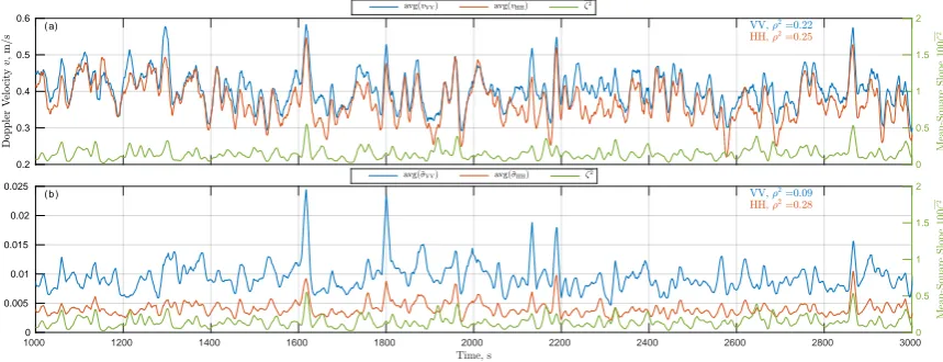
Figure 4.Time series of (top panel) DV and (bottom panel) NRCS. Green – mean-square slope, bold
blue/orange – VV/HH. Average interval is 10 s.
Some of previous hypotheses of the origin of LF radar variations involve wind turbulence [17].
118
Comparing time series of LF DV and NRCS with LF wind speed (Fig.2) suggests that the NRCS is
119
correlated with wind, while the DV is not. Alternative mechanisms of the origin of LF radar variations
120
involve wave group structure that modulates i) surface mean-square slope (MSS), which affects the LF
121
NRCS in accordance with the two-scale model,σ=σ(1+Pζ2)[18], ii) intermediate waves to which
122
shorter parasitic waves are bounded (LF DV mechanism, [19]), iii) wave breaking inhomogeneity [21]
123
that imprints on sub-peak frequency variability of both DV and NRCS [20].
124
As a proxy for wave group, we use the running slope variance, var(ζ) =ζ2, estimated from radar
125
DV. We compare this “running” MSS with average DV (Fig.4a) and wind-compensated NRCS, i.e.
126
NRCS from which wind-induced variations are removed, ˜σ=σ−aUn, where the wind exponentnis
127
set to 3 andais determined by the linear fit,σ=aUn(Fig.4b). The LF variations of DV and NRCS are
128
related to the running mean MSS, but to a lesser extent than to the wind speed. As expected from the
129
two-scale model e.g. [18], HH NRCS is stronger affected by MSS than VV NRCS.
130
Linear correlation analysis suggests that wind accounts for∼30% of the total LF NRCS (slower
131
than 10 s) variance, while only 10% (30%) of the residual, non-wind-induced, variance is accounted for
132
by MSS variations at VV (HH) polarization, respectively.
In contrast, LF DV weakly correlates with the wind, however∼20% of its variance is explained
134
by MSS variations. Notice, that the correlation between DV and MSS is also affected by the fact that the
135
MSS is retrieved from the DV itself (WG data are not used because they were measured far from the
136
radar footprint). DV-based MSS proxy accounts only for waves longer than the radar footprint length
137
that don’t respond to immediate wind fluctuations, which in turn explains rather low correlation
138
between MSS and wind.
139
6. Non-Linear Transfer Function 140
A non-zero correlation between MSS and LF NRCS reflects a non-linearity of NRCS-wave slope
141
transfer. In general, a non-linear transfer results in spectrum broadening by leaking energy into
142
multiple order harmonics and sub-harmonics [27,28]. Our focus is on the latter as a potential cause of
143
observed LF features in both NRCS and DV.
144
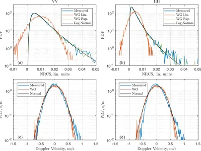
The impact of non-linearity is demonstrated by the shape of NRCS probability density function
145
(PDF, Fig. 5a,b) that is strongly skewed and has a non-Gaussian shape. If a linear MTF is used to
146
retrieve the NRCS from observed wave slopes, which have quasi-Gaussian PDF, the PDF of retrieved
147
NRCS is obviously quasi-Gaussian, in contrast with the observed PDF.
148
Because the characteristic magnitude of the linear MTF is significant (≈10−20), even small wave slopes produce NRCS variations comparable in magnitude to the NRCS itself. As an alternative, a non-Linear MTF (NLMTF) can be used [29,30]
σ=σ0exp(Mζ), (9)
to which the traditional linear MTF (7) is the first order approximation.
149
For the normally distributed slopesζ, the NRCS given by eq. (9) is log-normally distributed:
p(σ) =p(σ(ζ))
dζ
dσ
= q 1
2πζ2Mσ
exp
(
−log
2(
σ/σ0)
2M2ζ2 )
. (10)
Since the “non-linear” NRCS is non-Gaussian, theσ0-parameter is not the mean NRCS,σ, but
they are related:
σ0=σexp
(
−M
2ζ2
2
)
. (11)
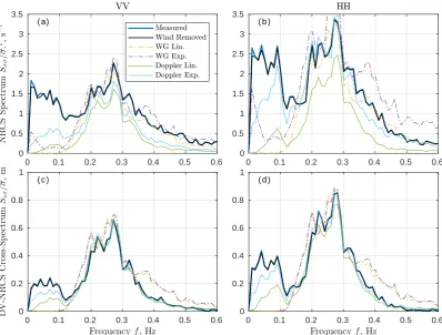
The PDF of observed NRCS is approximated well by a log-normal distribution eq. (10) as shown
150
in Figs. 5a,b. Observed NRCS spectra and DV-NRCS cross-spectra are also reproduced well using
151
the NLMTF (Fig.6). As expected, the linear MTF doesn’t produce LF components if applied to WG
152
data. Switching to NLMTF makes LF spectral level non-zero but still lower than in observations. LF
153
components are produced if the DV is used as a wave probe and the linear MTF is applied. Indeed,
154
it reflects the presence of LF components in measured DV. Finally, if DV-based wave elevations are
155
non-linearly transformed into the NRCS, the simulated co- and cross-spectra have well pronounced LF
156
features.
157
The difference between measured and wind-compensated NRCS spectra is small suggesting that
158
near surface and anemometer height wind variations are not well correlated at 0.01 Hz< f <0.1
159
Hz. Our wind detection setup was primarily designed to control the background atmospheric
160
conditions, i.e. record-mean wind velocity. The measurement height (21-m height) as well as wind
161
vane anemometer sampling rate (0.2 Hz) both are not optimal to detect 0.01−0.1 Hz wind fluctuations,
162
which may be associated with the atmospheric boundary layer perturbations produced by wave
163
groups confined to lower heights, which are simply missed by 21-m height sensor. Due to the above
164
wind detection limitations, it might be not surprising to see such weak impacts of observed wind
165
fluctuations on NRCS spectra in the LF range (Fig.6).
-0.01 0 0.01 0.02 0.03 0.04 0.05 10-1
100 101 102
( a)
-0.01 0 0.01 0.02 0.03 0.04 0.05 10-1
100 101 102
( b )
-1.5 -1 -0.5 0 0.5 1 1.5
10-2 10-1 100
( c )
-1.5 -1 -0.5 0 0.5 1 1.5
10-2 10-1 100
( d )
Figure 5.Probability density function (PDF) of (a,b) NRCS and (c,d) DV for (a,c) VV polarization and
0 0.1 0.2 0.3 0.4 0.5 0.6 0
0.5 1 1.5 2 2.5 3 3.5
( a)
0 0.1 0.2 0.3 0.4 0.5 0.6 0
0.5 1 1.5 2 2.5 3 3.5
( b )
0 0.1 0.2 0.3 0.4 0.5 0.6 0
0.2 0.4 0.6 0.8 1
( c )
0 0.1 0.2 0.3 0.4 0.5 0.6 0
0.2 0.4 0.6 0.8 1
( d )
Figure 6.Measurements and various estimates of (a,b) NRCS spectra and (c,d) DV-NRCS spectra for
On the other hand, the DV PDF is quasi-Gaussian (Fig. 5c,d) indicating that measured DV is
167
reproduced well by WG data using the linear MTF (with the exception of HH polarization for which
168
the PDF is a slightly skewed). Hence, LF DV variations cannot be explained by the NLMTF. However,
169
the DV measured by a radar is footprint-averaged local DV weighted by local NRCS. Because the
170
local NRCS is a non-linear function of local wave slopes, the measured DV is affected by non-linearity
171
of NRCS transfer function. In other words, the observed LF DV signatures can result from NRCS
172
non-linearity that is involved through the footprint averaging.
173
It is also surprising that DV-based surface elevation works better than in-situ WG data for radar
174
spectra estimates (Fig. 5). This fact may be related to distortions of apparent frequency of shorter
175
waves by orbital velocity of longer waves, in turn suggesting that WG-based frequency attribution
176
of wave elevation is not reliable at high frequencies. Next we will perform a numerical simulation to
177
overcome a lack of information on unresolved short waves.
178
7. Numerical Simulation 179
To model one-dimensional moving surface, a semi-empirical wavenumber KMC spectrum [31,32]
180
is used. The length of simulated domain is 400 m (≈10 dominant wavelengths). Spatial resolution
181
0.05 m corresponds to the shortest wavelength. The initial surface is a superposition of harmonics
182
with amplitudes obeying the KMC spectrum and phases randomly distributed over[0; 2π]interval.
183
The phase speed of each harmonic is determined by the dispersion relation,c=p
g/k+γk, where
184
γ = 7.3×10⁻⁵N/m is the surface tension. All harmonics propagate towards an upwind looking
185
radar oriented atθ=48◦incidence angle. Simulation lasts for 12 hours (about 10000 dominant wave
186
periods) with 0.1 s time step.
187
The local NRCS is computed using NLMTF from the local surface slope (gradient), while the local
188
DV is a sum of orbital velocities of all harmonics. The radar NRCS and DV are footprint averages:
189
σ(t) =
Z
σ(x,t)W(x)dx/
Z
W(x)dx (12)
v(t) =
Z
v(x,t)σ(x,t)W(x)dx/
Z
σ(x,t)W(x)dx (13)
whereW(x)is the Gaussian-shaped two-way antenna pattern. We will explore different values of
190
W(x)half-width, including 4m width that corresponds to our radar footprint.
191
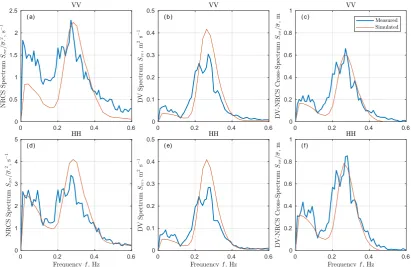
Simulated DV and NRCS spectra, and their cross-spectra are shown in Fig. 7 along with
192
measurements. Given rather simple 1-D surface elevation model, the overall consistency between
193
measurements and simulations is remarkably good. The simulated DV peak level is higher than in
194
observations because all wave energy is directed into a single direction, while the real spectrum is not
195
unidirectional. The simulation nicely reproduces the LF signatures for all spectra with the exception of
196
VV NRCS (Fig.7a). This can be explained by the presence of LF wind variability (not accounted for
197
by this simple 1-D model) to which VV NRCS is more sensitive due to higher contribution of Bragg
198
backscattering. VV cross-spectrum (Fig.7a) is reproduced better than NRCS spectrum indicating that
199
wind-induced variability is important for NRCS and to much lesser extent for DV.
200
Although the hydrodynamics MTF responsible for short-long wave correlation is not directly
201
included in the simulation, its impact on LF variations is partially present through the using of
202
observed MTF magnitude (M=12−16), which otherwise would be lower for the tilting only.
203
8. The Role of Non-Linearity 204
The simulated 1-D surface is used to evaluate the importance of non-linear radar imaging effects.
205
First, we test how good the linear MTF approximation (7) is, if the actual transfer function is non-linear
206
(9). The DV and NRCS are simulated using the NLMTF with the magnitude varying from 1 to
207
40. Footprint half-widthW(x)in (12,13) is set to 1 m to increase the footprint cut-off frequency of
208
simulated spectra. Based on simulated NRCS and DV, the linear MTF is estimated using (8).
0 0.2 0.4 0.6 0
0.5 1 1.5 2 2.5
( a)
0 0.2 0.4 0.6
0 0.1 0.2 0.3 0.4 0.5
( b )
0 0.2 0.4 0.6
0 0.2 0.4 0.6 0.8 1
( c )
0 0.2 0.4 0.6
0 1 2 3 4 5
( d )
0 0.2 0.4 0.6
0 0.1 0.2 0.3 0.4 0.5
( e)
0 0.2 0.4 0.6
0 0.2 0.4 0.6 0.8 1
( f )
Figure 7. Simulated and measured (a,d) NRCS, (b,e) DV, (c,f) DV-NRCS spectra for (top row) VV
polarization and (bottom row) HH polarization.
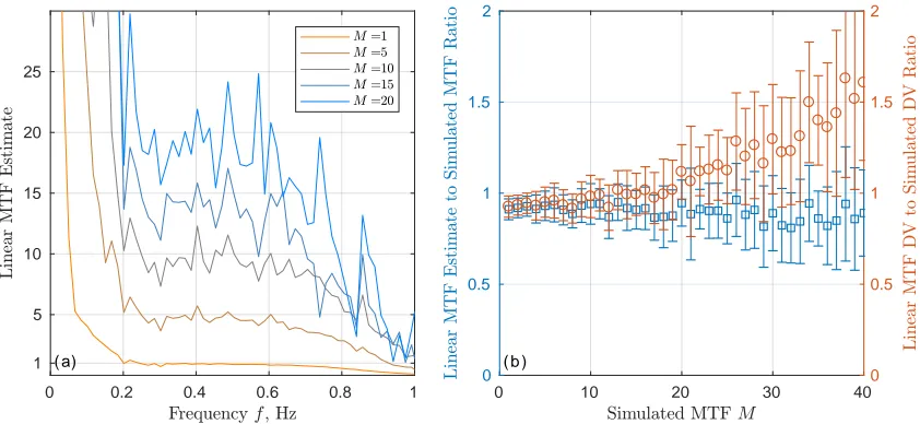
The estimated magnitude of linear MTF (Fig.8a) equals the original MTF magnitude,|M|, for
210
fp< f < f1with the upper frequency, f1, determined by the footprint size. The linear MTF estimate 211
level averaged over[0.2; 0.6]Hz frequency interval is close (to within 10% error corridor) to the original
212
MTF magnitude forM<20 (Fig.8b, blue symbols), although its uncertainty increases at higher|M|.
213
The time mean DV, or the DV averaged over the whole wave spectrum, is also estimated from linear MTF and known wave spectrum using (5,7):
V=vσ/σ=g−1Re{G∗M
Z
ω3Szz(ω)dω}=g1/2Re{G∗M
Z
k3/2Szz(k)dk} (14) The ratio of DV estimate (vσ/σ) based on linear MTF (14) to DV estimate based on non-linear
214
MTF (13) is close to 1 for|M|<20 to within 10% error (Fig.8b). For the majority of practical cases
215
(excluding near-threshold winds and largeθwith M>20 [23]), the impact of non-linear effects on
216
radar DV can be ignored. One simplification made forDVestimation (14) is the using of frequency
217
independent MTF, which is not the case for swell that has higher MTF due to wave-induced wind
218
variations [2,33], which are not included in our simple simulations. Thus our numerical simulations
219
suggest that linear MTF (7) is a good approximation for non-linear MTF (9) given small long wave
220
slopes.
221
9. Summary 222
This study presents the analysis of LF variations of Doppler radar backscattering from the sea
223
surface based on a Ka-band field measurements. They are separated by applying the running 10-s mean
224
roughly corresponding to double period of dominant waves. A specialized laboratory experiment was
225
conducted to estimate the measuring system noise and to prove that it is not the cause of observed LF
226
variations. LF winds explain about∼30% of LF NRCS variance, while LF DV does not correlate with
227
LF winds. Non-wind-induced NRCS is partly explained by LF mean-square slope (10% / 30% for VV /
228
HH polarization, respectively) indicating non-linear transfer between slopes and NRCS.
0 0.2 0.4 0.6 0.8 1 1
5 10 15 20 25
( a)
0 10 20 30 40
0 0.5 1 1.5 2
0 0.5 1 1.5 2
( b )
Figure 8.(a) Linear MTF estimated using (8) based on non-linearly simulated NRCS for variousMin
(9). (b) Ratio of linear MTF estimate (8) averaged at 0.2 Hz<f <0.6 Hz toM(left y-axis) and ratio of DV estimate based on linear MTF (14) to DV simulated using non-linear MTF (13, right y-axis).
As deducted from the sample distribution analysis, the local NRCS is essentially a non-linear
230
function of wave slopes in line with previous studies [27–30]. This non-linearity explains observed
231
NRCS spectra, including their LF part, if non-linear MTF is applied to wave slopes estimated from
232
instantaneous radar DV (orbital velocity). The DV has quasi-Gaussian distribution (positive tails are
233
caused by wave breaking) indicating that it is a linear function of surface slopes. Hence, LF variations
234
in radar DV is a consequence of spatial averaging that is a product of the local DV weighted by the
235
local non-linear NRCS.
236
Impact of nonlinearity of radar measurements is tested using a 1-D surface elevation simulation
237
based on the semi-empirical wave spectrum [31] corresponding to observed wind and wave fetch. If
238
the NRCS is modeled using a non-linear transfer function, the measured DV and NRCS spectra are
239
adequately reproduced by the simulation even though the hydrodynamics effects are not included.
240
Simulated LF variance of VV NRCS is underestimated by a factor of≈2 suggesting that wind variability,
241
which is not included in the simulation, is still important. However, the DV-NRCS cross-spectrum is
242
simulated well even without the inclusion of wind variability effect. This suggests that LF DV is not
243
strongly affected by LF winds, which impact can be ignored for the time mean DV.
244
The relationship between the LF radar variation and the non-linearity of modulation transfer
245
function may explain other available observations. In particular, the magnitude of LF variations in
246
the L-band are almost twice as large as in the X-band [17]. This is explained by larger L-band MTF
247
magnitude (e.g. see Fig. 11 in [34]) that results in more pronounced nonlinearity. The increase of LF
248
level of DV spectra at large incidence angles [19,20] is explained by larger radar footprint size and by
249
larger MTF magnitude caused by hydrodynamics modulation of wedge scattering.
250
Simulations with different MTF magnitudes show that MTF nonlinearity has little effect on
251
estimated linear MTF as well as on estimated time mean DV. This confirms that traditional linear MTF
252
[1,3] is a good approximation for real non-linear radar MTF, while LF signatures are “artifacts” caused
253
by MTF nonlinearity and spatial averaging over finite radar footprint.
254
Acknowledgments: The core support of the work was provided by Russian Science Foundation grant
255
No. 17-77-10052. Field experiments were supported by FASO of Russia under the State Assignment (No.
256
0827-2018-0002). Sea surface simulation was supported by the Ministry of Science and Education (Goszadanie
257
5.2928.2017/PP) and NASA/PhO. The authors would like to thank Anton Garmashov of MHI for providing
258
standard meteorological measurements.
Author Contributions:V.K. and Yu.Yu. conceived and designed the experiments; V.K., B.C. and S.G. provided
260
sea surface model for numerical simulations; Yu.Yu. performed the experiments, analyzed the data, and wrote the
261
paper.
262
Conflicts of Interest:The authors declare no conflict of interest.
263
Abbreviations 264
The following abbreviations are used in this manuscript:
265
DV Doppler Velocity FFT Fast Fourier Transform
HH Horizontal Transmit-Receive Polarization LF Low Frequency
MSS Mean-Square Slope
MTF Modulation Transfer Function
NLMTF Non-Linear Modulation Transfer Function NRCS Normalized Radar Cross-Section
PDF Probability Density Function
VV Vertical Transmit-Receive Polarization UTC Coordinated Universal Time
WG Wave Gauge
266
267
1. Keller, W.C.; Wright, J.W. Microwave scattering and the straining of wind-generated waves. Radio Science
268
1975,10, 139–147. doi:10.1029/RS010i002p00139.
269
2. Schröter, J.; Feindt, F.; Alpers, W.; Keller, W.C. Measurement of the ocean wave-radar modulation transfer
270
function at 4.3 GHz. J. Geophys. Res. (Oceans)1986,91, 923–932. doi:10.1029/JC091iC01p00923.
271
3. Plant, W.J. The Modulation Transfer Function: Concept and Applications. Radar Scattering from Modulated
272
Wind Waves1989, pp. 155–172.
273
4. Goldstein, R.M.; Zebker, H.A. Interferometric radar measurement of ocean surface currents. Nature1987,
274
328, 707–709. doi:10.1038/328707a0.
275
5. Romeiser, R.; Thompson, D.R. Numerical study on the along-track interferometric radar imaging
276
mechanism of oceanic surface currents. IEEE Trans. Geosci. Remote Sens. 2000, 38, 446–458.
277
doi:10.1109/36.823940.
278
6. Martin, A.; Gommenginger, C. Towards wide-swath high-resolution mapping of total ocean surface
279
current vectors from space: Airborne proof-of-concept and validation. Remote Sensing of Environment2017,
280
197, 58–71. doi:http://dx.doi.org/10.1016/j.rse.2017.05.020.
281
7. Chapron, B.; Collard, F.; Ardhuin, F. Direct measurements of ocean surface velocity from space:
282
Interpretation and validation. J. Geophys. Res. (Oceans)2005,110, 7008. doi:10.1029/2004JC002809.
283
8. Johannessen, J.A.; Chapron, B.; Collard, F.; Kudryavtsev, V.; Mouche, A.; Akimov, D.; Dagestad, K.F. Direct
284
ocean surface velocity measurements from space: Improved quantitative interpretation of Envisat ASAR
285
observations. Geophys. Res. Lett.2008,35, 22608. doi:10.1029/2008GL035709.
286
9. Mouche, A.A.; Collard, F.; Chapron, B.; Dagestad, K.F.; Guitton, G.; Johannessen, J.A.; Kerbaol, V.; Hansen,
287
M.W. On the Use of Doppler Shift for Sea Surface Wind Retrieval From SAR.IEEE Trans. Geosci. Remote
288
Sens.2012,50, 2901–2909. doi:10.1109/TGRS.2011.2174998.
289
10. Bourassa, M.A.; Rodriguez, E.; Chelton, D. Winds and currents mission: Ability to observe
290
mesoscale AIR/SEA coupling. Proc. Int. Geosci. Remote Sens. Symp., 2016, pp. 7392–7395.
291
doi:10.1109/IGARSS.2016.7730928.
292
11. Ardhuin, F.; Aksenov, Y.; Benetazzo, A.; Bertino, L.; Brandt, P.; Caubet, E.; Chapron, B.; Collard, F.; Cravatte,
293
S.; Dias, F.; Dibarboure, G.; Gaultier, L.; Johannessen, J.; Korosov, A.; Manucharyan, G.; Menemenlis, D.;
294
Menendez, M.; Monnier, G.; Mouche, A.; Nouguier, F.; Nurser, G.; Rampal, P.; Reniers, A.; Rodriguez, E.;
295
Stopa, J.; Tison, C.; Tissier, M.; Ubelmann, C.; van Sebille, E.; Vialard, J.; Xie, J. Measuring currents, ice drift,
296
and waves from space: the Sea Surface KInematics Multiscale monitoring (SKIM) concept. Ocean Science
297
Discussions2017,2017, 1–26. doi:10.5194/os-2017-65.
12. Bao, Q.; Lin, M.; Zhang, Y.; Dong, X.; Lang, S.; Gong, P. Ocean Surface Current Inversion
299
Method for a Doppler Scatterometer. IEEE Trans. Geosci. Remote Sens. 2017, 55, 6505–6516.
300
doi:10.1109/TGRS.2017.2728824.
301
13. Rodriguez, E.; Wineteer, A.; Perkovic-Martin, D.; Gál, T.; Stiles, B.; Niamsuwan, N.; Rodriguez Monje,
302
R. Estimating Ocean Vector Winds and Currents Using a Ka-Band Pencil-Beam Doppler Scatterometer.
303
Remote Sens.2018,10(4), 576. doi:10.3390/rs10040576.
304
14. Nouguier, F.; Chapron, B.; Collard, F.; Mouche, A.; Rascle, N.; Ardhuin, F.; Wu, X. Sea Surface Kinematics
305
From Near-Nadir Radar Measurement. IEEE Trans. Geosci. Remote Sens.2018. accepted.
306
15. Fois, F.; Hoogeboom, P.; Le Chevalier, F.; Stoffelen, A. An analytical model for the description of
307
the full-polarimetric sea surface Doppler signature. J. Geophys. Res. (Oceans)2015, 120, 988–1015.
308
doi:10.1002/2014JC010589.
309
16. Yurovsky, Y.Y.; Kudryavtsev, V.; Grodsky, S.A.; Chapron, B. Normalized Radar Backscattering Cross-section
310
and Doppler Shifts of the Sea Surface in Ka-band. 2017 Progress in Electromagnetic Research Symposium
311
(PIERS); , 2017. in press.
312
17. Plant, W.J.; Keller, W.C.; Cross, A. Parametric dependence of ocean wave-radar modulation transfer
313
functions. J. Geophys. Res. (Oceans)1983,88, 9747–9756. doi:10.1029/JC088iC14p09747.
314
18. Grodsky, S.A.; Kudryavtsev, V.N.; Bol’shakov, A.N.; Smolov, V.E. Experimental investigation of fluctuations
315
of radar signals caused by surface waves.Physical Oceanography2001,11, 333–352. doi:10.1007/BF02509228.
316
19. Plant, W.J. A model for microwave Doppler sea return at high incidence angles: Bragg scattering from
317
bound, tilted waves. J. Geophys. Res. (Oceans)1997,102, 21131–21146. doi:10.1029/97JC01225.
318
20. Hwang, P.A.; Sletten, M.A.; Toporkov, J.V. A note on Doppler processing of coherent radar backscatter
319
from the water surface: With application to ocean surface wave measurements. J. Geophys. Res. (Oceans)
320
2010,115, n/a–n/a. C03026, doi:10.1029/2009JC005870.
321
21. Donelan, M.; Longuet-Higgins, M.S.; Turner, J.S. Periodicity in whitecaps. Nature1972,239, 449–451.
322
doi:10.1038/239449a0.
323
22. Yurovsky, Y.Y.; Kudryavtsev, V.N.; Grodsky, S.A.; Chapron, B. Ka-Band Dual Copolarized Empirical
324
Model for the Sea Surface Radar Cross Section. IEEE Trans. Geosci. Remote Sens. 2017,55, 1629–1647.
325
doi:10.1109/TGRS.2016.2628640.
326
23. Yurovsky, Y.Y.; Kudryavtsev, V.N.; Chapron, B.; Grodsky, S.A. Modulation of Ka-band Doppler Radar
327
Signals Backscattered from the Sea Surface. IEEE Trans. Geosci. Remote Sens. 2018, pp. 1–19. in press,
328
doi:10.1109/TGRS.2017.2787459.
329
24. Toba, Y.; Koga, M. A parameter describing overall conditions of wave breaking, whitecapping, sea-spray
330
production and wind stress. InOceanic Whitecaps; Monahan, E.C.; Niocaill, G.M., Eds.; Reidel Publishing
331
Company, 1986; pp. 37–47.
332
25. Jessup, A.T.; Melville, W.K.; Keller, W.C. Breaking waves affecting microwave backscatter 1. Detection and
333
verification.J. Geophys. Res. (Oceans)1991,96, 20547–20559. doi:10.1029/91JC01993.
334
26. Thompson, D.R.; Jensen, J.R. Synthetic aperture radar interferometry applied to ship-generated internal
335
waves in the 1989 Loch Linnhe experiment. J. Geophys. Res. (Oceans)1993,98, 10259–10270.
336
27. Hesany, V.; Moore, R.K.; Gogineni, S.P.; Holtzman, J.C. Slope-induced nonlinearities on imaging of ocean
337
waves. IEEE J. Oceanic Eng.1991,16, 279–284. doi:10.1109/48.90884.
338
28. Schmidt, A.; Bao, M. The modulation of radar backscatter by long ocean waves: A quadratically nonlinear
339
process? J. Geophys. Res. (Oceans)1998,103, 5551–5562. doi:10.1029/97JC00634.
340
29. Trunk, G.V. Radar Properties of Non-Rayleigh Sea Clutter.IEEE Transactions on Aerospace and Electronic
341
Systems1972,AES-8, 196–204. doi:10.1109/TAES.1972.309490.
342
30. Gotwols, B.L.; Thompson, D.R. Ocean microwave backscatter distributions. J. Geophys. Res. (Oceans),
343
99, 9741–9750. doi:10.1029/93JC02649.
344
31. Kudryavtsev, V.N.; Makin, V.K.; Chapron, B. Coupled sea surface-atmosphere model: 2. Spectrum of short
345
wind waves. J. Geophys. Res. (Oceans)1999,104, 7625–7639. doi:10.1029/1999JC900005.
346
32. Yurovskaya, M.V.; Dulov, V.A.; Chapron, B.; Kudryavtsev, V.N. Directional short wind wave spectra derived
347
from the sea surface photography. J. Geophys. Res. (Oceans)2013,118, 4380–4394. doi:10.1002/jgrc.20296.
348
33. Alpers, W.; Ross, D.; Rufenach, C. On the detectability of ocean surface waves by real and synthetic
349
aperture radar.J. Geophys. Res. (Oceans)1981,86, 6481–6498.
34. Feindt, F.; Schroeter, J.; Alpers, W. Measurement of the ocean wave-radar modulation transfer function
351
at 35 GHz from a sea-based platform in the North Sea. J. Geophys. Res. (Oceans)1986,91, 9701–9708.
352
doi:10.1029/JC091iC08p09701.