Extreme Learning Machine for Robustness

Article

1

Extreme Learning Machine for Robustness

2

Enhancement of Gas Detection Based on

3

Tunable Diode Laser Absorption Spectroscopy

4

WENHAI JI 1_{, LI ZHONG} 1_{, YING MA} 1_{, DI SONG} 1_{, XIAOCUI LV} 1_{, CHUANTAO ZHENG} 2_,

5

GUOLIN LI 1,_*

6

1 _{College of Information and Control Engineering, China University of Petroleum, Qingdao 266580, China}

7

2 _{State Key Laboratory on Integrated Optoelectronics, College of Electronic Science and Engineering, Jilin}

8

University, Changchun, 130012, China

9

* Correspondence:[email protected]; Tel.: +86-532-86980953

10

11

Abstract: In this work, a tailored extreme learning machine (ELM) algorithm to enhance the overall

12

robustness of gas analyzer based on the tunable diode laser absorption spectroscopy (TDLAS)

13

method is presented. The ELM model is tailored through activation function selection, input weight

14

and bias searching, and cross validation method to address the analyzer robustness issues for

15

industrial process analysis field application. The two particular issues are the inaccurate gas

16

concentration measurement caused by the process gas background components variation, and the

17

inaccurate spectra shift calculation caused by spectral interference. By using our algorithm, the

18

concentration error is reduced by one order of magnitude over a much larger stream pressure and

19

component range compared with that obtained by classical least square (CLS) fitting methods based

20

on reference curves. Additionally, it is shown that with our algorithm, the wavelength shift accuracy

21

is improved to less than 1 count over 1000 counts spectra length. In order to test the viability of our

22

algorithm, a trace ethylene (C2H4) TDLAS analyzer with coexisting methane was implemented, and

23

its experimental measurements support analyzing robustness enhancement effect.

24

Keywords: gas analyzers; optical sensors; TDLAS; extreme learning machine

25

26

1. Introduction

27

Absorption spectroscopy is a versatile technique to obtain fundamental physics parameters with

28

great precision. Tunable diode laser absorption spectroscopy (TDLAS) technology has gained

29

popular acceptance for trace gas measurement in various industries due to rapid development of

30

optoelectronics technology. Because of its high sensitivity and fast response time, it is widely used in

31

coal mine safety [1], combustion measurement [2], petrochemical process analysis [3], dissolved gas

32

detection [4], gas emission and air quality monitoring [5] etc.

33

But there are challenges to maintain the analyzing robustness and accuracy for long term onsite

34

industrial applications. The conventional concentration measurement method is based on calibration

35

model using reference spectra [6, 7]. The common issues are spectral deformation and spectral

36

interference caused by process background and operating condition variation. These factors are

37

entangled in real time measurement due to the dynamic nature of industrial process. The analyzing

38

system deviates from the original calibration and its performance degrades over time. To address

39

these issues, linear regression algorithms such as classical least square fitting (CLS, also known as

40

multiple linear regression -MLR) method [6], partial least square fitting (PLS) method [7] are

41

commonly adopted in TDLAS spectra analysis. CLS algorithm is also named as reference curve

42

method. PLS is an integration of regression and principle component analysis. The models are good

43

for certain tolerance of background change.

44

But when the spectral interference or deformation becomes stronger, it is hard to achieve

45

satisfactory performance with the linear regression algorithms. Then nonlinear algorithms such as

46

artificial neural networking (ANN) [8], supporting vector machine (SVM) [9] and extreme learning

47

machine (ELM) [10-15] were introduced in spectra analysis. Among those, ELM is a novel single layer

48

forward neuro networking (SLFN) algorithm proposed and developed by G. Huang [16-20]. It has

49

the relative advantages of simple structure and less computation time. ELM is capable of regression

50

and classification [21-22]. For the classification application, ELM was used in coal classification [10],

51

dynamic fresh fruit detection [11], and traffic road signs identification [22] etc. The regression ELM

52

for quantitative calculation was applied in element analysis [12], gas concentration retrieval [13],

53

stellar star abundance calculation [14], diesel fuel and blend oil analysis [15], and food extrusion

54

processing [23] etc. ELM spectra analysis [10-15] was used in micro-NIR, Fourier transform infrared

55

(FTIR) spectroscopy, laser induced breakdown spectroscopy (LIBS) area. Its application in TDLAS

56

spectra analysis for industrial process analysis was not implemented so far.

57

2. Experiment

58

The process of TDLAS analyzer gas concentration measurement is shown in Figure. 1. The

59

spectra generation process is illustrated in Figure. 1 (a). The second harmonic component of laser

60

absorption was obtained through laser current modulation and demodulator extraction. The

61

procedure of calibration model training and verification is illustrated in Figure. 1(b) and (c).

62

However, in the practical model verification, there are challenges due to the harsh operating

63

environment. Particularly, we will deal with two issues. First issue is the accurate gas concentration

64

prediction caused by background components and gas pressure variation during process

65

measurement. Second issue is the accurate spectra shift prediction with strong spectral interference.

66

The direct impact is the degradation of prediction accuracy, shown by the error band width d change

67

from ideal case to practical case in Figure. 1(c). ELM was proposed to address the challenges. With

68

ELM, we aim to calculate both the gas concentration in dynamical process background and the actual

69

spectra shift with the interfering spectral structures.

70

We choose trace ethylene (C2H4) measurement as the application example. C2H4 is an important

71

indicator gas which needs real time monitoring at ppmv (part per million by volume, default as ppm)

72

level in many areas. For example, in the biomedical area, analyzing C2H4 in breath air can be used to

73

study lipid peroxidation of human body cell, so that related deases can be diagnosed at early stages.

74

Another example is monitoring coal spontaneous combustion which is a major risk in the coal mining

75

wells and storages [24-25]. Trace level C2H4 is produced in early stages and the concentration

76

increases as the process continues. CH4 is a common coexisting component and also brings spectra

77

interference. So, accurate measurement of C2H4 concentration at trace level is difficult.

78

Accordingly, 0-200ppm range C2H4 measurement experiment was designed with 0-2000ppm

79

CH4 presence and in dynamic environment. The system schematic is shown in Figure. 2. A

Cortex-80

A5 chip manufactured by Atmel is used as the master micro controller unit (MCU). The A5 MCU

81

controls a commercial module PCI-FPGA-1A manufactured by Port City Instruments (PCI). Its main

82

functions are laser wavelength scan, modulation, photoelectric current amplification and

83

demodulation. A sawtooth shape driving current is applied to the distributed feedback (DFB) laser

84

to scan the wavelength. The tuning range is around 0.45 nm which covers two absorption peaks of

85

the C2H4 at 1626.35nm and 1626.53nm respectively. The laser temperature is stabilized and adjusted

86

by a WTC3293 module (TEC, temperature controller). The scan period is 102ms and the maximum

87

out of fiber power is 3.3mW. The laser driving current is superimposed with a 31.4 KHz sin wave AC

88

signal (1f) for amplitude modulation. The transmitted light is collected by a PIN InGaAs detector.

89

The photon current is directed sequentially through I/V convertor, preamplifier, band pass filter, and

90

phase sensitive lock-in amplifier (demodulator). The second harmonic component denoted as 2f is

91

generated by using a frequency doubled reference signal (2f Ref) in demodulator. The modulation

92

synthesizer (DSS). The optical power signal during the scan denoted as DC is obtained through a low

94

pass filter. DC and 2f, together with gas status parameter temperature T and pressure P are feed to

95

the A5 processor through an analog to digital convertor (ADC).

96

(b) Model training

(c) Model verification (1) Ideal case

(2) Practical case

Spectral interference Frequency drift Calibration Model Calibration Model Y 200 ... 100

0 500 1000

-2500 0 2500 5000 Am pl it ud e( a. u. ) Wavelength(a.u.)

0 500 1000

-2500 0 2500 5000 Am pl it ud e( a. u. ) Wavelength(a.u.)

0 500 1000

-2500 0 2500 5000 Am pl it ud e( a. u. ) Wavelength(a.u.) 200 100

0 500 1000

-2500 0 2500 5000 Am pl it ud e( a. u. ) Wavelength(a.u.) Calibration Model X Am p litu d e Wavelength Demodulator Detector Gas Cell

C2H4 CH4 N2 scanning

LD (a) Spectra generation

0 20 40 60 80 100 0 20 40 60 80 100 Set Pred ict ion

0 20 40 60 80 100 -20 0 20 40 60 80 100 120 Predict io n Set

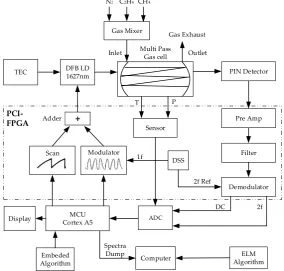
97

Figure 1. The process of TDLAS analyzer gas concentration measurement. (a) 2f spectra generation;

98

(b) Model training with training set; (c) Model verification with collected spectra.

99

DC 2f Outlet

Inlet Multi Pass Gas cell Gas Mixer N2 C2H4 CH4

TEC DFB LD

1627nm PIN Detector

Scan Modulator MCU Cortex A5 Display DSS Embeded Algorithm Computer ELM Algorithm + ADC Spectra Dump Adder Gas Exhaust T P Pre Amp Filter 2f Ref 1f Sensor PCI-FPGA Demodulator

100

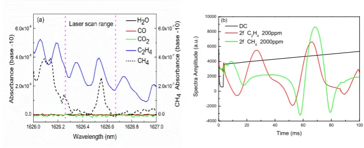
The C2H4 absorption features were thoroughly searched in the near infrared region [24, 26].

102

Absorbance of 1ppm-m moisture (H2O), carbon monoxide (CO), carbon dioxide (CO2), CH4 and C2H4

103

in 1626-1627nm wavelength region is depicted in Figure 3. (a). To demonstrate the clear features of

104

CH4 spectra, its absorbance is plotted on right axis whose scale is 10 times of left axis. At 25℃,

105

atmosphere pressure and 1ppm-m concertation level, the peak absorbance of CH4 is one magnitude

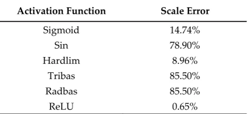
106

weaker than C2H4. The other potential components such as H2O, CO, and CO2 are four or more

107

magnitudes weaker than C2H4. Thus, from 1626.25nm to 1626.70nm region (defined by two magenta

108

dotted lines in Fig. 3(a)) is the ideal wavelength scan range for C2H4 analysis. Experimentally acquired

109

DC and 2f spectra of 200ppm C2H4 and 2000ppm CH4 balanced in N2 are shown in Figure. 3(b) and

110

used as the reference curve in CLS method. The spectral structure of C2H4 and CH4 are overlapped.

111

The gas stream is generated through an automatic gas mixing station with premixed 1000 ppm C2H4

112

in nitrogen (N2), 1% CH4 in N2 and pure N2 bottles.

113

To address the spectra analysis challenges, two experiments were designed. To prepare for

114

analyzer calibration model, test samples should be representative and cover all possible status. Thus,

115

the associated independent variables of the samples such as gas concentrations, pressure, laser

116

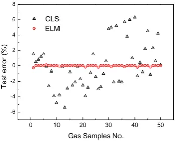
driving current etc. should be randomly set. The first experiment was the process simulation test,

117

where CH4 was mixed in stream. The C2H4, CH4 concentration, and gas pressure was randomly

118

varied through the Excel random function in experiment design. The second experiment was spectra

119

shift simulation test, where driving current was randomly adjusted with dynamic gas composition

120

to mimic spectra drift effect.

121

0 20 40 60 80 100

-4000 -2000 0 2000 4000 6000 8000 10000

DC

2f C₂H₄ 200ppm

2f CH₄ 2000ppm

S

pec

tr

a

A

m

pl

itu

de

(a

.u

.)

Time (ms)

(b)

122

Figure 3. (a) Absorbance of 1ppm-m H2O, CO, CO2, CH4 and C2H4 in 1626-1627nm wavelength

123

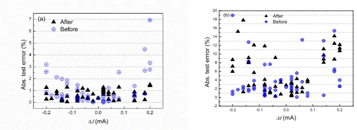
region. (b) Experimentally acquired DC and 2f spectra of 200ppm C2H4 and 2000ppm CH4.

124

2.1. Process Simulation Experiment

125

This experiment was to simulate the industrial process in a controlled scenario, where the C2H4

126

concentration, CH4 concentration and gas pressure varied during the measurement. Fifty mixing gas

127

streams were generated with C2H4 up to 200 ppm, CH4 up to 2000 ppm and balancing nitrogen. The

128

pressure was controlled in 900 to 1100 mbar range. Gas cell was maintained at room temperature. In

129

order to get representative test sample, the concentrations and pressure were randomly set. The 50

130

corresponding spectra are plotted in Figure. 4 (a). For an isolated spectra feature, the gas

131

concentration is proportional to the spectra peak height, which is the simple case of Beer-Lambert

132

law. But due to CH4 interference, accurate measurement can’t be obtained by direct counting the C2H4

133

spectra peak height.

134

2.2. Spectral Drift Simulation Experiment

135

A commercial analyzer can be used for 5-10 years. During its lifetime, spectra deformations are

136

unavoidable. Many factors lead to deformation, including the complex operating environment, the

137

spectra drift is the most common type and produces adverse impact on the calibration model

139

accuracy.

140

In this experiment, the gas cell pressure was fixed at 1000 mbar. The gas concentration was also

141

randomly set. The starting current was randomly set in between 59.8 mA to 60.2 mA. The variation

142

range was 0.4 mA and the peak shift range was around 16 counts over 1000 counts spectra range. The

143

current scanning range was fixed at 24 mA. Thus, there was no stretching or shrinking effect. The

144

collected spectra are shown in Figure.4 (b). For an isolated spectra feature, the spectra shift can be

145

calculated by peak tracking based on peak position difference between current spectrum and target

146

spectrum. But it is unlikely to get spectra shift by tracking any spectra peak for the overlapping

147

spectra structures in Figure. 4(b).

148

0 20 40 60 80 100

-4000 -3000 -2000 -1000 0 1000 2000 3000 4000 5000 6000

Process test spectra

S

p

ec

tr

a

A

m

plit

ud

e (

a.u.

)

Time (ms)

(a)

0 20 40 60 80 100

-4000 -3000 -2000 -1000 0 1000 2000 3000 4000 5000 6000

Drift test spectra

Spe

ctr

a

Am

pli

tud

e (

a

.u

.)

Time (ms) (b)

149

Figure 4. Spectra collected in the process simulation test (a) and in spectra drift simulation test (b).

150

3. ELM Algorithm Theory

151

ELM was originally developed for the single-hidden-layer feedforward neural networks and

152

then extended to the “generalized” SLFNs whose hidden layer need not be tuned [16–20]. Essentially,

153

ELM originally proposes to apply random computational nodes in the hidden layer, which are

154

independent of the training data. Different from traditional learning algorithms for a neural type of

155

SLFNs [16], ELM aims to reach not only the smallest training error but also the smallest norm of

156

output weights. ELM is identified with better training speed and generalization ability than BP neuro

157

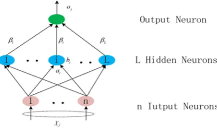
networking and SVM. The ELM algorithm structure is shown in Figure. 5.

158

Figure 5. Structure of ELM algorithm.

159

We target to improve the prediction accuracy of C2H4 concentration or spectra shift amount.

160

They are assigned as model output o. The prediction is based on the collected spectra. Other variables

161

such as gas temperature T and pressure P may also be helpful to improve prediction accuracy. They

162

are assigned as model input X.

163

1

( ) , 1, ,

L

i i j i j

i

g W X b o j N

β =

⋅ + = =



where β_i is the output weight, [ ₁, ₂, , ]T

i i i in

W _{= ω ω} _ω is input weight, X_j is the j-th input of

165

spectra sample X, g（ ） is the activation function, W X_i⋅ _jis the inner product，_bi is the bias of

166

the neuron,

o

167

hidden layer nodes, n is the input layer neuron number, the output layer neuron number is 1.

168

The goal of ELM model training is to find βi，Wi and bi to match the real output t with

169

model prediction o,

170

1

||

|| 0

N

j j

j

o

t

=

−

=



Let

171

1

( ) , 1, ,

L

i i j i j

i

g W X b t j N

β

= ⋅ + = =



or in matrix form,

H

_β

=

T

where，

172

1 1 1 1

1 1

( ) ( )

H

( ) ( )

L L

N L N L N L

g W X b g W X b

g W X b g W X b _×

⋅ + ⋅ +

 

 

=_{ }

 _{⋅ + ⋅ +} 

 



  



, ₍₅₎

As a result, the output weight is estimated after model training as,

173

^

-1 = ( T)

H T H HH T

β

Compared with SLFNs, the major difference of ELM is that the input weight matrix W and bias

174

matrix b of the hidden layer is randomly initialized. Only the number of hidden layer neurons L is to

175

be optimized. That’s why ELM is so distinct in its simple structure and fast learning speed. The

176

problem of low learning efficiency and tedious parameter setting of traditional ANN algorithm is not

177

an issue in ELM.

178

ELM optimization research was focused on kernel or excitation function selection [19],

179

progressing modelling and generic algorithm [23], priori parameter initialization [27], and particle

180

swarm optimization [28] etc. ELM model can be improved through optimizing the neuron numbers

181

L [16]. Due to the randomness of the input weight and threshold, there exists fluctuations in the final

182

output. Its stability and generalization ability could be further improved by generic algorithm (GA)

183

optimization of input weight W and bias b. GA is well known for searching of global optimized

184

parameter [23]. GA searching is done through many generations of selection, crossover and mutation

185

operation. Since GA is well studied, its detailed theory is not presented.

186

The activation function is also critical to the model performance in terms of model convergence

187

speed and predication accuracy. But there is no general rule of activation function selection. In neuro

188

networking algorithms, the popular activation function choices are sigmoid, tanh, and ReLU [29] etc.

189

The impact of activation function needs further study with experiment data.

190

To compare the performance of ELM, the conventional classical least square (CLS) fitting

191

method is introduced with following expression,

192

0 1 1 2 2

where Y is the collected spectra, R1 and R2are reference spectra，ai (i=1,2) is the corresponding

193

regression coefficient which is used to determine the gas concentration.

194

4. Algorithm model evaluation and discussion

195

4.1. Experimental Spectra Analysis Procedures

196

Spectra were analyzed with the following procedures: spectra collection, spectra pre-process,

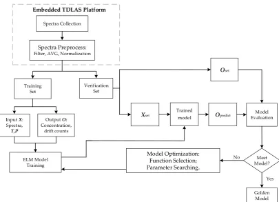
197

spectra partition, model training, model evaluation, model optimization, as shown in Figure. 6.

198

No

Yes Spectra Collection

Spectra Preprocess:

Filter, AVG, Normalization

Training Set

Verification Set

ELM Model Training

Model Evaluation

Meet Model?

Golden Model

Model Optimization: Function Selection; Parameter Searching.

Input X: Spectra,

T,P

Output O:

Concentration, drift counts

Oset

Embedded TDLAS Platform

Xset

Trained

model Opredict

199

Figure 6.Spectra analysis flow chart.

200

Spectra collection and pre-process is the first step and done in the embedded system. The

201

collected spectrum has 1000 data points. The spectra were averaged after 50 scans. They were further

202

smoothed by Savitzky–Golay (S-G) polynomial filter to improve the signal to noise ratio (SNR). To

203

cancel the effect of light power fluctuation on spectra strength, spectra were normalized by DC. The

204

PCI-FPGA module separates the spectra into the laser off null period and scan period. The

205

demodulation was done through software, it produces a delay in 2f spectra with respect to DC and

206

needs further alignment. So the region from 80 to 860 was selected for analysis to exclude null period

207

and trivial 0s from spectra alignment.

208

In spectra partition, they were divided into verification set and training set. A popular method

209

is the k-fold cross validation (CV). We take 5-fold CV as an example. Spectra were first labeled by

210

indices. They were separated into 5 subgroups per the remainder after the spectra index was divided

211

by 5. Spectra in 4 subgroups were used for model training. Spectra in the leftover subgroup were

212

used for verification. The 5 subgroups took turns to act as training and verification sets.

213

The model performance can be evaluated in many respects such as training time, computation

214

resources, prediction accuracy etc. For the gas analysis purpose, the accuracy is the most significant

215

(

)

_

_ _

i i i

i o t Scale Error Abs

Fs

Scale Error Max Scale Error

− =

=

（ ） _,

(8)

where o_i and t_i are the prediction and set values of the i-th spectrum in verification set, Fs is

217

the full measurement range. Depending the analyzing variables, the accuracy formula may take some

218

modifications. The spectra shift prediction was converted to the current changes in mA.

219

4.2. Process Simulation Test Analysis

220

The 50 spectra collected in the process simulation test are used to calculate the C2H4

221

concentration prediction in dynamic backgrounds with ELM model. There are several aspects that

222

effect the model performance, such as the function options and parameters value. It is done through

223

the following optimization step.

224

First, we study the effect of activation function with sigmoid, sin, hardlim, tribas, radbas and

225

rectified linear unit (ReLU) choices with subgroup 1 to 4 as training set and subgroup 5 as verification

226

set. The scale errors for different activation functions are listed in Table 1. The scale error for ReLU is

227

0.65% which is substantially better than other choices. By comparing the analytical expression of

228

different activation functions [29], we find that ReLU has linear expression and broad linear response

229

input range without saturation. In this research scenario, the spectra has linear or quasi-linear

230

response to concentration, pressure, temperature or drift variation in defined range. Thus, ReLU is

231

more favorable to the spectra analysis compared with other activation functions than other choices.

232

It is also faster in convergence and its behavior is closer to authentic biological neural activation

233

function. So ReLU is selected for future ELM model.

234

Table 1. Model performance indicated by scale error with different activation functions.

235

Activation Function Scale Error

Sigmoid 14.74% Sin 78.90% Hardlim 8.96%

Tribas 85.50% Radbas 85.50%

ReLU 0.65%

Then, the GA global searching is used to find optimum hidden layer neuron number L, input

236

weight W and bias b. In GA search setting, the group scale is 50, max generation is 25, crossover rate

237

is 0.93, and mutation rate is 0.05. L is optimized at 150. After W_bestand b_best are identified at

238

generation 12, the scale error is improved from 0.65% to 0.37%.

239

Finally, a 5-fold cross validation method is used for the model evaluation. In the validation, each

240

of the 5 groups take turns to act as verification set to test the model trained from the rest four groups.

241

Scale error of each test subgroup with corresponding ELM model is listed in Table 2. It is obvious

242

that ELM model built with subgroup 2-5 as training and subgroup 1 as verification has lowest scale

243

error 0.27%.

244

The optimized ELM models are obtained after GA parameter searching, activation function trial,

245

and 5-fold cross validation. The test error which is defined as prediction values subtract set value

246

normalized by the full range is plotted in Figure. 7(circle). The optimum ELM model is obtained with

247

ReLU activation function and with k=1 subgroup cross validation. The errors of training set are closer

248

to zero because they are deeply suppressed by the activation function during the model training

249

process in which the predication matches the set value as close as possible. The errors of 10 spectra

250

in verification set are larger than in training set. The ELM model performance is represented by max

251

253

Table 2. Scale error in each subgroup for CLS and optimized ELM models.

254

Subgroup CLS ELM

1 5.70% 0.27%

2 2.80% 0.40%

3 6.00% 0.46%

4 4.20% 0.57%

5 6.30% 0.37%

As comparison basis, CLS is introduced to obtain the C2H4 concentration. Its performance is

255

represented by the max error of 50 sample spectra. In CLS regression, R1 is taken with 200ppm C2H4

256

and R2 is taken with 2000ppm CH4. The scale error of CLS method for 50 spectra is listed in Table 2

257

with max error of 6.30%. The CLS test error is also plotted in Figure. 7 (triangle). From the Table 2

258

and Figure. 7, the error of ELM model is reduced by one order of magnitude than traditional CLS

259

method.

260

0 10 20 30 40 50

-6 -4 -2 0 2 4 6 8

CLS ELM

T

es

t erro

r (

%

)

Gas Samples No.

261

Figure 7. C2H4 concentration prediction errors vs gas samples for CLS method and optimized ELM model.

262

4.3. Spectral Drift Simulation Test Analysis

263

4.3.1. Spectra shift measurement with ELM model

264

The ELM algorithm was still utilized to obtain the actual spectral shift in the dynamic process.

265

After GA optimization and 5-fold cross validation, the neuron number is 170 and the activation

266

function is ReLU. In the modelling C2H4 concentration is replaced by spectral shift in the model. The

267

scale error is defined as the current prediction error divided by the 16 counts variation range. The

268

scale errors for subgroups are listed in Table 3.The best model corresponding to scale error of 4% is

269

ELM model trained by subgroup 1,2,4,5. The spectra shift prediction error is 4%×16= 0.64 count.

270

In conventional peak tracking method, spectra shift is monitored the by tracking the peak with

271

least spectral interference. So the right C2H4 peak is selected. The scale error of each subgroup is listed

272

in Table 3. Due to concentration variation and residue CH4 interference, the precision and accuracy

273

of spectra wavelength shift calculation is much worse than ELM method. The max error is 100% and

274

16 counts.

275

Table 3. Scale error of spectra shift calculation in each subgroup for peak tracking and ELM.

Subgroup Peak Tracking ELM

1 -56% -16%

2 -75% -15%

3 69% 4%

4 63% 10%

5 -100% 5%

4.3.2. Prediction error after shift correction

277

After the spectra shift obtained through peak tracking and ELM model, the spectra can be

278

backshifted. The purpose is to match the shifted spectra with calibration spectra so that original

279

calibration model is still valid. The C2H4 concentration prediction error with and without backshift

280

correction are calculated with previously obtained optimum ELM model and CLS method. The result

281

is shown in Figure. 8 (a) and (b).

282

-0.2 -0.1 0.0 0.1 0.2 -2

0 2 4 6 8 10 12 14 16 18 20

After Before

A

bs

.

tes

t errror (%)

ΔΙ (mA)

(b)

283

Figure 8. C2H4 concentration prediction abs. error vs. current shift with and w/o shift correction. (a) ELM

284

method (b) peak tracking method.

285

The scale error of C2H4 concentration for each spectrum is plotted against ΔI，

286

set 60 I I

Δ = − , (9)

where I_set is the setting current, 60 mA is the base current. Before correction, the error pattern

287

demonstrates a V shape. The explanation is that as spectra shifts more, the error increase more. After

288

ELM correction, the error patterns demonstrate flat belt shape. The belt widths are greatly shrunk.

289

The error is improved from 6.92% to 1.50%. For peak tracking and CLS method, the error has no

290

obvoius improvement. This is due to the fact of very inaccurate peak shift calculation. The

291

improvement of spectra shift correction with ELM method is demonstrated.

292

5. Conclusions

293

In this paper, ELM were employed in the TDLAS spectra analysis. Two experiments were carried

294

out with trace C2H4 measurement as the application example. In the process simulation test, not only

295

the C2H4 and CH4 concentration were varied, but also the gas pressure was controlled in 900 to 1100

296

mbar range. For optimized ELM model, scale error of C2H4 concentration is obtained at 0.27% with

297

ReLU activation function, GA optimization of input neuron number L, input weight W and bias b,

298

and 5-fold cross validation. For traditional CLS method, the scale error is 6.30%.

299

In the spectra shift simulation test, ELM and peak tracking method are used to analysis the

300

spectra shift. The prediction errors of spectra shift are less than 1 count for ELM and 16 counts for

301

peak tracking. Then the spectra were back shifted to match with the calibration. The C2H4

302

reduced from 6.92% to 1.50% by ELM method after shift correction. There is no noticeable error

304

improvement with peak tracking and CLS method. The errors remain in 20% range.

305

In a summary, the optimized ELM model has demonstrated dramatic improvement of TDLAS

306

prediction accuracy by one order of magnitude in the trace C2H4 measurement in a simulated

307

industrial process analysis scenario. The robustness enhancement is explicit. ELM algorithm could

308

be extended to other areas of spectra analysis in the harsh application environments and dynamic

309

process background. Complicated spectra deformation in addition to spectra shift could be dealt with

310

ELM algorithm for future research.

311

Author Contributions: Conceptualization, Wenhai Ji and Guolin Li; methodology, Wenhai Ji and Li Zhong;

312

software, Ying Ma and Xiaocui Lv; validation, Di Song; formal analysis, Ying Ma; investigation, Li Zhong;

313

writing—original draft preparation, Wenhai Ji.; writing—review and editing, Chuantao Zheng and Guolin Li.

314

Funding: This research received funding from Natural Science Foundation of China (Nos. 61775079, 61627823),

315

Natural Science Foundation of Shandong Province (No. ZR2017LF023), Key Science and Technology R&D

316

program of Jilin Province (No. 20180201046GX), Huimin Special Project of Qingdao Science and Technology

317

Bureau (No. 17-3-3-89-nsh), Jilin University State Key Laboratory on Integrated Optoelectronics Open Research

318

Fund Project (No. IOSKL2017KF0).

319

Conflicts of Interest: The authors declare no conflict of interest. The funders had no role in the design of the

320

study; in the collection, analyses, or interpretation of data; in the writing of the manuscript, or in the decision to

321

publish the results.

322

References

323

1. Y. Wei.; J. Chang.; J. Lian.; et al. A Coal Mine Multi-Point Fiber Ethylene Gas Concentration Sensor. Photonic

324

Sensors 2015, 5(1), 67-71.

325

2. D. Shi.; W. Song.; J. Ye.; et al. Experimental Investigation of Reacting Flow Characteristics in a Dual-Mode

326

Scramjet Combustor. International Journal of Turbo & Jet-Engines 2016, 33(2), 95-104.

327

3. Y. Wang.; Y. Wei.; J. Chang. Tunable Diode Laser Absorption Spectroscopy Based Detection of Propane for

328

Explosion Early Warning by Using a Vertical Cavity Surface Enhanced Laser Source and Principle

329

Component Analysis Approach. IEEE Sensors Journal 2017, 17, 4975-4982.

330

4. J. Jiang.; M. Zhao.; G.-M. Ma.; H.-T. Song.; C.-R. Li.; X. Han.; C. Zhang. TDLAS-Based Detection of

331

Dissolved Methane in Power Transformer Oil and Field Application. IEEE Sensors Journal 2018, 18,

2318-332

2325.

333

5. Z. Yuan.; X. Yang.; W. Xie.; X. Li. Research on the Online Test of Diesel NOx Emission by TDLAS.

334

Spectroscopy and Spectral Analysis 2018, 38, 194-199.

335

6. H. Li.; Y. Zhu.; F. Dong.; et al. Simulation Design and Verification of CO Monitoring Based on Tunable

336

Diode Laser Absorption Spectroscopy. Precision Electromagnetic Measurements (CPEM) 2010 Conference

337

on. IEEE, 2010, 482-483.

338

7. Y. Wang.; Y. Wei.; T. Liu.; et al. TDLAS Detection of Propane/Butane Gas Mixture by Using Reference Gas

339

Absorption Cells and Partial Least Square Approach. IEEE Sensors Journal 2018, 18(20), 8587-8596.

340

8. P. Barmpalexis.; A. Karagianni.; I. Nikolakakis.; K. Kachrimanis. Artificial Neural Networks (ANNs) and

341

Partial Least Squares (PLS) Regression in The Quantitative Analysis of Cocrystal Formulations by Raman

342

and ATR-FTIR Spectroscopy. Journal of Pharmaceutical and Biomedical Analysis 2018, 158, 214-224.

343

9. C. Malegori.; E. J. Nascimento Marques.; S. T. de Freitas.; M. F. Pimentel.; C. Pasquini.; E. Casiraghi.

344

Comparing the Analytical Performances of Micro-NIR and FT-NIR Spectrometers in the Evaluation of

345

Acerola Fruit Quality, Using PLS and SVM Regression Algorithms. Talanta 2017, 165, 112-116.

346

10. B. Le.; D. Xiao.; Y. Mao. Coal. Classification Based on Visible, Near-Infrared Spectroscopy and CNN-ELM

347

Algorithm. Spectroscopy and Spectral Analysis 2018, 38, 2107-2112.

348

11. Y. Yang.; S. Zhang.; Y. He. Dynamic Detection of Fresh Jujube Based on ELM and Visible/Near Infrared

349

Spectra. Spectroscopy and Spectral Analysis 2015, 35, 1870-1874.

350

12. T. Owolabi.; M. Gondal. Development of Hybrid Extreme Learning Machine Based Chemometrics for

351

Precise Quantitative Analysis of LIBS Spectra Using Internal Reference Pre-Processing Method.

352

ANALYTICA CHIMICA ACTA 2018, 1030, 33-41.

13. Y. Chen.; Z. Wang.; Z. Wang.; X. Li. Research on Concentration Retrieval of Gas FTIR Spectra by Interval

354

Extreme Learning Machine and Genetic Algorithm. Spectroscopy and Spectral Analysis 2014, 34, 1244-1248

355

.

356

14. Y. Bu.; G. Zhao.; J. Pan.; Y. Bharat Kumar. ELM: an Algorithm to Estimate the Alpha Abundance from

Low-357

resolution Spectra. Astrophysical Journal 2016, 817, 78.

358

15. X. Bian.; C. Zhang.; X. Y. Tan.; M. Dymek.; Y. Guo.; L. Lin.; B. Cheng.; X. Hu. Boosting Extreme Learning

359

Machine for Near-Infrared Spectral Quantitative Analysis of Diesel Fuel and Edible Blend Oil Samples.

360

Analytical Methods 2017, 9, 2983-2989.

361

16. G. Huang.; Q. Zhu.; C. Siew. Extreme Learning Machine: A New Learning Scheme of Feedforward Neural

362

Networks. In Proceedings of the IEEE International Conference on Neural Networks, Budapest, Hungary,

363

25-29 July 2004; 985-990.

364

17. G. B. Huang.; Q. Y. Zhu.; C. K. Siew. Extreme Learning Machine: Theory and Applications.

365

Neurocomputing 2006, 70, 489-501.

366

18. G. B. Huang.; D. H. Wang.; and Y. Lan. Extreme Learning Machines: A Survey. International Journal of

367

Machine Learning & Cybernetics 2011, 2, 107-122.

368

19. G. B. Huang. An Insight into Extreme Learning Machines: Random Neurons, Random Features and

369

Kernels. Cognitive Computation 2014, 6, 376-390.

370

20. G. B. Huang.; H. Zhou.; X. Ding.; R. Zhang. Extreme Learning Machine for Regression and Multiclass

371

Classification. IEEE Trans Syst Man Cybern B Cybern 2012, 42, 513-529.

372

21. X. X. Yin.; S. Hadjiloucas.; J. He.; Y. Zhang.; Y. Wang.; D. Zhang. Application of Complex Extreme Learning

373

Machine to Multiclass Classification Problems with High Dimensionality. Digital Signal Processing 2015,

374

40, 40-52.

375

22. Z. Huang.; Y. Yu.; J. Gu.; H. Liu. An Efficient Method for Traffic Sign Recognition Based on Extreme

376

Learning Machine. IEEE Transactions on Cybernetics 2016, 47, 920-933.

377

23. R. J. Kowalski.; C. Li.; G. M. Ganjyal. Optimizing Twin-Screw Food Extrusion Processing through

378

Regression Modeling and Genetic Algorithms. Journal of Food Engineering 2018, 234, 50-56.

379

24. W. D. Pan.; J. W. Zhang.; J. M. Dai.; Y. F. Zhang. Tunable Diode Laser Absorption Spectroscopy for

380

Simultaneous Measurement of Ethylene and Methane near 1.626 μm. Journal of Infrared & Millimeter

381

Waves 2013, 32, 486-490.

382

25. F. V. D. Schoor.; F. Verplaetsen. The Upper Explosion Limit of Lower Alkanes and Alkenes an Air at

383

Elevated Pressures and Temperatures. Journal of Hazardous Materials 2016, 128, 1-9.

384

26. S. W. Sharpe.; T. J. Johnson.; R. L. Sams.; P. M. Chu.; G. C. Rhoderick.; P. A. Johnson. Gas-phase Databases

385

for Quantitative Infrared Spectroscopy. Applied Spectroscopy 2004, 58, 1452-1461.

386

27. K. Javed.; R. Gouriveau.; N. Zerhouni. SW-ELM: A Summation Wavelet Extreme Learning Machine

387

Algorithm with A Priori Parameter Initialization. Neurocomputing 2014, 123, 299-307.

388

28. F. Han.; M. R. Zhao.; J. M. Zhang.; Q. H. Ling. An Improved Incremental Constructive Single-Hidden-Layer

389

Feedforward Networks for Extreme Learning Machine Based on Particle Swarm Optimization.

390

Neurocomputing 2016, 228,133-142.

391

29. C. Yeom.; K. Kwak. Short-Term Electricity-Load Forecasting Using a TSK-Based Extreme Learning

392