A 2D spatial light modulator for spatio temporal shaping

(1)

(2)

(3)

(4)

(5)

Spatio-temporal phase shaping

Light is our primary means of observing the universe. Sunlight scatters off the objects around

us, showing us the world we live in. At night, on the open sea, one is treated to the most

beautiful celestial views, with light coming from stars at unintelligible distances away from

us. Now we want to use light as a tool, not in its raw form, but harnessed and sculptured, to

see things previously beyond our reach. We lit up the dark when we learnt to harness fire,

and nowadays we can control light in more fundamental ways, to illuminate the universe on a

molecular scale. In this thesis, we will show how light can be manipulated and shaped into the

extreme forms required for this, and we will demonstrate some of the applications.

Shaping light is done with a Spatial Light Modulator (SLM). For this project a novel two

dimensional SLM was bought and implemented. Chapter 2 discusses the different types of

two dimensional Spatial Light Modulators available and the considerations made in choosing

the newly bought SLM. The implementation and calibration of the SLM is described in

Chap-ters 3 and 4, in the spatial and spectral domain, respectively. Several new calibration

(8)

2

Chapter 1: Spatio-temporal phase shaping

we present a unique application of a two dimensional SLM with an in situ FROG setup that

contains no moving parts. Finally, Chapter 6 focusses on the algorithms underlying the

op-timisation experiments in which SLMs are often used. New insights in the coupling between

the SLMs and the driving algorithms are presented, including a novel parameterisation that

improves the optimisations.

This chapter will continue with an introduction in the world of shaping light. We will start

with the spectral domain, in which we manipulate different colours separately. Then the

spa-tial domain is discussed, and we end with some potenspa-tial applications of the combination of

spatial and spectral shaping of light.

1.1 Spectral shaping

Molecular processes occur on a time range of femtoseconds to nanoseconds. These processes

include such things as the interaction between molecules in chemical reactions, the folding of

proteins into different configurations, and the excitation and subsequent fluorescent emission

of dyes. In order to influence these systems we must interact with them at these time scales.

Pulses of light only a few tens of femtoseconds long, allow us to manipulate and steer

molec-ular interactions. However, even the most simple molecules exhibit intricate behaviour that

places extreme demands on the nature of the light with which it interacts. In order to effect a

desired response, light must be tailored very specifically to manipulate the interaction of light

and matter.

It is the field of coherent control that busies itself with controlling physical systems on

a quantum mechanical level through interaction with light. By shaping the light so that its

temporal signature matches the development of the system under scrutiny, it is possible to

steer processes and gain insight in their nature.1

For one, we can use this control that we have over molecules to effect a certain result.

As an example of this we can look at photodynamic therapy,2wherein cancer cells are

selec-tively treated by a photosensitizer: a drug that only becomes active through excitation with

light. By specifically tailoring the excitation light to the dynamics of this photosensitizer, we

can increase its efficiency and reduce unwanted side effects. For this, precise control over the

temporal profile of the excitation light is a necessity.

Secondly, we can use the interaction of light with molecules to gain further insight into the

workings of the molecules. While these systems are too complex to understand a priori, we

(9)

Section 1.1: Spectral shaping

3

Figure 1.1: The addition of sinusoidal waves with varying frequencies. If a broad spectrum of frequencies is combined, an ultrashort pulse is the result.

excite the molecules with specific and well defined light pulses.3

Evidently, we need precise control over the temporal characteristics of our light pulses in

order to manipulate systems on a femtosecond or picosecond timescale. This is known as

spectral (or temporal) shaping of light. For an extensive treatise on spectral shaping the reader

is referred to the review article of Weiner.4Here, only an attempt is made to give the reader an

intuitive understanding of spectral shaping.

1.1.1 Femtosecond light pulses

Forgoing a debate on the wave-particle duality of light, let us picture light as a wave with a

certain amplitude and frequency. The amplitude gives the intensity of the light while the

fre-quency defines its colour. A single colour would then give us one continuous sinusoidal wave,

but what happens if we combine a broad range of colours, as in Fig. 1.1?

Where the waves of all the colours simultaneously reach their peak value, we find a peak

in our intensity. However, when we look at our beam of light slightly before or after this peak

intensity, we see the intensity drop quickly. As the frequencies of all colours differ slightly, the

total contribution of the different colours does not amount to much at several tens of

fem-toseconds from the peak intensity. Some are at the peak of a vibration, while others are in a

trough. Summed up, we see that there is only a short pulse in time wherein all the colours

interfere constructively. In fact, the more colours we add, the shorter this pulse becomes.

If we thus want to make a pulse that is as short as possible — and remember that we need

a very short pulse to interact with the fast vibrations of the molecules — then we must have a

(10)

4

Figure 1.2: Analogy between the acoustic and optical domain. The staff describes the time and frequency characteristics of the music. Similarly, we can describe a pulse of light in time and frequency. Figure adapted from Ref. 3.

time, then it will consist of many different colours.

1.1.2 A melody of light

We now know that ultrashort pulses have a broad spectrum (i.e. it consists of many different

colours). So how does this permit us to shape this pulse in time? This question is most easily

answered with a musical analogue to light.

While light is an electromagnetic vibration where different frequencies represent different

colours, sound is a vibration of air where each pitch has a unique frequency. The

representa-tion of a sinusoidal wave with an amplitude and frequency holds in both cases.

In music, each frequency is represented by a note on a musical score. Fig. 1.2 shows such

a musical score, with the pitch varying as we move up on the staff and time progressing as we

read the notes from left to right.

The femtosecond pulse that was described before, can be represented in the musical

ana-logue as hitting all the keys on a piano at once. This will produce a short burst of sound with a

lot of energy, but very little melody. If we want to make music, then we have to shift the notes

with respect to each other.

The simplest “music” that we might play, would be to slide a hand across the piano, striking

all the keys one after another. On a musical score, this is represented by placing the notes one

after another, going up in frequency as we move from left to right across the keys. With our

ears, we will also hear the pitch go up as we move up the musical scale. Crucial, is the delay

between the notes which shifts the low and high pitch in time.

(11)

Section 1.1: Spectral shaping

5

of notes in which he plays with the length of the notes, their combinations, their amplitudes,

and most importantly, the delays between them. If this is done right, then Beethoven’s Fifth

symphony or the national anthem of the Republic of Palau will emerge.

With light we can do the same. As said, key is the delay between the different notes or,

better said, between the different frequencies. If we look back to Fig. 1.1, then we see that

a specific point in time was chosen where all colours are simultaneously at the peak of their

vibration. The phase (delay) between the different colours is zero and we obtain a single burst

of light, just like when hitting all the keys of a piano at once.

Playing with the relative phases of the different colours allows us to create not a musical

melody, but a “melody” of light. A sweep across the musical scale is a chirped pulse in the

optical domain: the red light precedes the blue, just as the low pitch precedes the higher notes

or vice versa. More complicated phase differences can give rise to higher order chirp, pulse

trains, or light pulses that are specifically tailored to specific molecules.

Let us consider the musical analogue once more. Occasionaly, a particularly skilful

musi-cian may compose an exceptionally good song. In fact, it is even possible to alter someone’s

mood and to play on someone’s emotions with the right music. Maybe you go out dancing and

get in a party mood with the latest disco hit or you wind down after a stressful day with your

favourite mellow pop song. It requires a very specific composition of notes to elicit an

emo-tional response. We can say that this music is tailored to a specific “vibration” and provides

control over your emotional processes.

With light we now aim to do the same thing. Not with emotions, but rather with molecules.

While we may not be able to make a molecule cry or giddy with joy, we can influence a chemical

reaction, break an intramolecular bond, or selectively excite a certain molecular marker. It is

towards this goal that we employ spectral phase shaping.

1.1.3 Experimental setup

One question is left unanswered: how do we manipulate the phase of light? For this, we have

a spatial light modulator (SLM). We want to apply a delay in time (corresponding to a shift in

phase) to a ray of light. Two ways exist of doing this, but before we look into this we must first

(12)

6

Figure 1.3: A 4f zero dispersion pulse compressor. The incident pulse is dispersed on a grating, separating the colours. Each colour is focussed onto an SLM pixel by the positive lens. In a transmissive setup as displayed here, the right half exactly mirrors the left half, thereby recombining the pulse after the second grating.

4f zero dispersion pulse compressor

Figure 1.3 shows a 4f zero dispersion pulse compressor.4The operation of this setup is

three-fold.

The incident femtosecond pulse is first divided into its separate frequency components

with a grating. The workings of a grating are slightly different, but the end result is similar to

that of a prism: every colour component is reflected off the grating at a slightly different angle,

thus converting a spectral difference (frequency) into a spatial difference (angle).

The second optical element is a positive lens which has two functions. One is to collimate

the beam coming off the grating so that it can later be recombined into one pulse. More

im-portantly, it focusses each colour onto a separate pixel on the SLM. This will allow us to then

manipulate each colour individually. Precisely how this manipulation is achieved we will find

out in the next section.

The third aspect of this setup is that it recombines all the colours back into one pulse. This

is achieved by the right half of Fig. 1.3, which is the precise mirror image of the left half. Shown

in Fig. 1.3 is a so-called transmissive setup wherein the light is manipulated as it is transmitted

through the SLM. Alternatively, a reflective setup can be used, using an SLM that reflects the

light. In that case, the light is automatically recombined as it retraces its path through the

focussing lens and past the grating.

If we remove the SLM from the setup, then we in no way alter the light as it passes through

the setup and we obtain the exact same pulse at the output as we put in. Also of note is the

distance between the various optical elements, which should be precisely the focal lengthf of

(13)

Section 1.2: Spatial shaping

7

So how does the SLM work? We have separated the spectrum and each colour is incident

on a different part of the SLM. With what magic is modulation of phase achieved?

Liquid crystal displays

A liquid crystal display (LCD) — as used in flatscreen computer monitors, telephone displays,

and digital alarm clocks — is a very commonplace example of a spatial light modulator. Light

from a backlight is first polarized and then passed through a liquid crystal (LC) which rotates

the polarization. The amount of rotation is regulated by applying a voltage over the LC. A

second polarizer at the front of the display then makes the intensity dependent on the driving

voltage.

For our application we are looking for phase modulation and not amplitude modulation.

Pure phase modulation can also be obtained using LCs, though some customization is

re-quired. In a normal LCD the liquid crystal is a so called twisted nematic LC whichtwists

the polarization. An alternative — and more expensive — form of nematic LCs is the

paral-lel aligned nematic variety. Here the polarization is left intact and applying a voltage over the

LC will change the refractive index for one polarization direction. By slowing down the light,

we can thus apply a phase shift as a function of a driving voltage. This gives us a phase-only

spatial light modulator.

Liquid crystal based SLMs can be used both in transmissive and reflective setups. The

electrodes in LCDs are transparent, thus allowing light to pass through. A reflective coating

can be added if a reflective setup is desired. Liquid crystal on silicon (LCoS) devices are only

usable in reflective setups as they have an opaque silicon backplane.

Deformable mirrors

An alternative method of phase modulation makes use of deformable mirrors. In a reflective

4f setup, we can also induce phase delay by physically changing the path length of the various

colours. In a deformable mirror, the surface of the mirror is deformed, thereby increasing or

decreasing the distance traversed by different parts of the spectrum.

1.2 Spatial shaping

Apart from manipulating light in time, we can also shape it in space using a spatial light

mod-ulator. While we are concerned with the phase delay as a function of frequency in spectral

(14)

8

Figure 1.4: With spatial shaping, the SLM shapes the phase of the wavefront. Far from the SLM (in the far-field) this transforms into an amplitude modulation. With a non-intuitive phase mask, complicated figures can be made, such as the Optical Sciences logo. So, what is the point?

Spatial shaping is nothing other than the manipulation of a beam profile. A glass lens is a

simple example of a two dimensional “phase mask” used for spatial shaping: different parts of

a beam incident on a lens will travel through different lengths of glass, thereby focussing the

beam onto the focal plane.

A more complicated spatial shaping process occurs on a grating. Diffraction off the regular

pattern of the grating causes a collimated incoming beam to be sent off into multiple

diffrac-tion orders. In general, this is the process that applies to all forms of spatial shaping. The

familiar terms of Fresnel and Fraunhofer diffraction apply.

An example is given in Fig. 1.4. On the SLM, a non-intuitive phase mask is displayed, which

manipulates the wavefront of the incident light. The intensity is left unchanged. Far from the

SLM — in the aptly named far-field — we obtain a complicated diffraction pattern. Given the

proper phase mask, we can even create highly complex images.

In short, we can create complicated scattering patterns on a two dimensional SLM to

spa-tially modulate a beam. An incoming monochromatic beam can be transformed into a wildly

scattered, inhomogeneous beam profile by applying a complicated phase mask. The inverse

is then also true: highly complex spatial distortions can be compensated using an SLM. This

is the concept by which adaptive optics in astronomical telescopes can compensate for

atmo-spheric distortions. It is even possible to compensate the incalculable distortions occurring in

highly turbid media such as bone, teeth, or egg shells.5

1.3 Applications of spatio-temporal phase shaping

A few recent examples of spatio-temporal shaping — the combination of shaping in the

spec-tral and spatial domains — will be discussed here, as well as some yet untested ideas.

(15)

spear-Section 1.3: Applications of spatio-temporal phase shaping

9

headed by the research groups of Nelson and Silberberg. They have recently presented some

proof-of-concept experiments wherein one dimension of the SLM is used for spectral shaping

of femtosecond pulses, while the second dimension is given various different uses.

Feurer and co-workers6presented proof-of-concept spatio-temporal shaping already in

2002. Across the spatial dimension of their SLM they created different pulse trains in time,

resulting in an image appearing in an unusual space-time plot. The limitation of the

spa-tial shaping to one dimension appears to severely limit applications of this technique to the

creation of funny images, as fervently shown by Vaughan.7

A more serious application of a two dimensional SLM was presented by Gundogdu and

co-workers8in 2007, in the dubiously named paper “Multidimensional coherent spectroscopy

made easy”. In this work, they physically divide one incident beam into four beams on the

SLM, spreading the spectrum in one dimension with a grating, and separating the four beams

along the spatial dimension. The four separately shaped beams are then combined in a

BOX-CARS setup to provide two dimensional spectra.

Frumker and Silberberg9used an identical device as used in the work of this thesis to shape

both amplitude and phase. By applying a grating in the spatial dimension of the SLM, they can

selectively attenuate their spectrum. The spectrum diffracts part of the incoming light into

higher orders which is not coupled back at the output of their shaper setup. In this way, they

can use a phase-only SLM for both phase and amplitude modulation. In related work,10they

added a scanning mirror that walked the beam across the spatial dimension of the SLM. By

applying different phase masks along the spatial dimension, they could greatly increase the

perceived refresh rate of their SLM. They report refresh rates of about 140 kHz, three orders of

magnitude greater than achievable with regular liquid crystal SLMs.

The main advantages named in the aforementioned applications all stem from the fact

that a single incident beam can be used for the same purposes where several separate laser

beams were originally required. By subdividing one beam on the SLM, one obtains a setup

that is easy to align, has an inherent phase relation between the various beams, and allows for

arbitrary waveform generation in all beams. Another possible application of two dimensional

SLMs that offers these same advantages is presented in this work in Chapter 5. There, we

demonstrate a single beam FROG setup with no moving parts which allows for quick and easy

characterisation of complicated waveforms at the sample position.

All applications of spatio-temporal shaping with a single two dimensional SLM are

(16)

10

Figure 1.5: Spatio-temporal pulse shaping can be either (a) uncoupled or (b) coupled.

is generally insufficient if the spatial characteristics of the system being studied are relevant.

However, systems that operate in only one spatial dimension do exist, and some (limited)

ap-plications of spatio-temporal shaping may exist here. One might consider, for example, the

excitation and propagation of surface plasmons, or the propagation of light in photonic

wave-guides. Whether spatio-temporal shaping has any real applications in the world of surface

plasmons remains to be seen, as — to the knowledge of the author — no such research has

been performed.

1.3.1 Smart CARS

Real spatio-temporal shaping where the light is shaped in two spatial dimensions to

accom-modate the spatial characteristics of the sample is more easily done using separate shapers for

both the spatial and spectral domains. An example of such a system11, would be the

combi-nation of chemically selective imaging through shaped CARS12(coherent anti-Stokes Raman

spectroscopy) with resolution enhancement and compensation for wavefront distortions with

spatial shaping.5

By tailoring the excitation pulses in CARS to the vibrations of specific molecules, or

pos-sibly even the specific folding-configurations of proteins, excellent chemical selectivity in

mi-croscopy can be obtained.12This may in the future allow for imaging cell processes in vivo.

Spatial shaping has been proven to allow for compensation of severe scattering in turbid

media and can even provide focussing within these media.5This should then also be possible

(17)

Section 1.3: Applications of spatio-temporal phase shaping

11

Combining the spatial and spectral shaping may in the future allow for chemical selective

imaging of biologically relevant processes within cell tissue or, in other words, deep within

human tissue. Apart from imaging, very local excitation of photosensitizers (previously

men-tioned in Section 1.1) may lead to unintrusive treatment of skin ailments.

The precise implementation of spatio-temporal shaping using multiple shapers will

re-quire significant study. As shown in Fig. 1.5, the straightforward combination of spectral and

spatial shaping will lead to uncoupled spatio-temporal shaping wherein the spatial and

spec-tral shaping are always separable. Preferably, the pulse can be shaped not just both in time

and space, but uniquely shaped in time at every point in space, and shaped in space at every

unique point in time. This will require coupling of the spatial and spectral shaping, for example

(18)

(19)

2

2D Spatial Light Modulators

Several design parameters were defined for the selection of a two dimensional spatial light

modulator. First, we had the need for a very large bandwidth, preferably from 400 up to 900nm.

Secondly, only phase-only modulators were considered with as little parasitic amplitude

mod-ulation as possible. Finally, a minimum of a few hundred uniquely addressable pixels in each

dimension were required to assure sufficient resolution for the creation of more complicated

pulse shapes.

This chapter lists the main manufacturers of two dimensional liquid crystal based SLMs,

as well as deformable mirrors. The given information is accurate per September 2007.

Consid-ering the rapid advances in SLM technology — especially in the field of deformable mirrors —

the use for the reader of this information in selecting a new SLM may be limited.

2.1 Liquid crystal displays

Liquid crystal based two dimensional SLMs are produced by only a few companies. The

(20)

14

Chapter 2: 2D Spatial Light Modulators

different products will be discussed here separately. The information given in this chapter

comes from both the websites of the manufacturers, as well as from telephone and e-mail

con-versations with their engineers and sales people. Their contact details are given in Appendix A.

2.1.1 Hamamatsu

In 2007, Hamamatsu introduced a new two dimensional SLM labelled the Programmable Phase

Modulator (PPM). The PPM consists of a parallel aligned nematic liquid crystal (PAL-SLM)

which is optically addressed with an LCD. The LCD at the back obviously has pixels, but the

LC at the front of the device which applies the phase modulation, has no pixel structure. This

means that there is less diffraction and you get a continuous shaping of your light. Whereas

a normal LCD is driven electrically, the PAL-SLM changes its optical properties when a

write-light is shone on it from the back. The pixelated write-light coming from the LCD is therefore swrite-lightly

defocused and shone on the PAL-SLM where it is converted into a phase modulation. It should

be noted that even though there are no pixels on the LC, there is a limit on the resolution of

the device. The LC cannot be modulated over shorter ranges than 10–20µm, regardless of the

write-light setup used. Moreover, Hamamatsu does not look favourable upon replacing the

original write light setup with a custom built one.

The PPM has a resolution of 1024 by 768 pixels and has standard bandwidths of 100 nm

in a range from 350 to 1600 nm for which a 2πphase shift is guaranteed. Custom devices can

be made with a maximum bandwidth of up to 350 nm. The restriction on the bandwidth is

caused by the need to have both a good anti-reflection coating at the front as well as a mirror

at the back of the device. The delivery time for a custom device is around 4 months for a price

exceedinge22.000,=. The Hamamatsu device is the only 2D LC-SLM with a 100% fill factor.

2.1.2 Boulder Nonlinear Systems

Boulder Nonlinear Systems (BNS) offers the XY Phase Series spatial light modulators in 5

va-rieties. Given our pulses with a central wavelength of 800 nm, only the model P512-0785 is

relevant. This device has a wavelength range of 760 to 865 nm. This range can potentially

be extended slightly, but at a loss of phase-resolution for the extended part of the spectrum.

Unique for the BNS device is the possibility of adding a dielectric mirror coating on top of the

electrical contacts at the back of the LC. This extends the fill factor to 100% and thus mitigates

the negative side-effects of a pixelated device. However, this extra coating does reduce the

(21)

Section 2.2: Deformable mirrors

15

50 addressable levels per pixel for a 2πphase shift. The refresh rate is around 18 Hz, which

is three times less than the other available phase shapers which operate at 60 Hz. Delivery

times of this SLM are up to 6 weeks, though reduced delivery times of 2 weeks are occasionally

possible. The estimated cost of a device wase20.000,=.

2.1.3 Holoeye

Holoeye has a large range of spatial light modulators, but only in the second half of 2007 did

they introduce a phase only modulator. This is the HEO1080p spatial light modulator with an

amazing resolution of 1920 by 1080 pixels with 8 bit addressing. This is only slightly smaller

than the largest SLM on the market which has 1920 by 1200 pixels and is also produced by

Holoeye. This high resolution does come at a cost: the fill factor is only 87%. While this is

good for pixelated devices, it will lead to significant amplitude loss which will not occur with

the devices of Hamamatsu and BNS. The bandwidth of the HEO1080p is officially given as

420–810 nm, but the device should also still be useful at slightly higher wavelengths. Other

groups have already used this SLM with 30 fs pulses centred at 800 nm. A 2_πphase shift is

guaranteed across the whole advertised wavelength range. The Holoeye device has a delivery

time of 4 weeks at a price ofe15.000,=.

2.2 Deformable mirrors

In the field of astronomy, deformable mirrors are the norm for wavefront correction. The

sur-face of a mirror is actively shape, thereby changing the path length of reflecting light. This

translates into a phase shift and thus these devices can be used for all forms of spatial and

spectral phase shaping. Both pixelated devices, as well as mirrors with a continuous flexible

membrane are available.

The mechanical nature of these shapers limit the number of actuators to a few hundred or

thousand, although rapid advances in microelectromechanical systems (MEMS) have led to

the recent introduction of a 200 by 240 pixel micro mirror device by the Fraunhofer Institute

for Photonic Microsystems. This same company also sells a 1 megapixel device for use in

in-dustrial lithography, but this SLM is only usable in the UV. The pixel stroke — the maximum

displacement of each pixel — is also limited to 180 (nm), which would equate to less than half

(22)

16

Chapter 2: 2D Spatial Light Modulators

2.3 Our choice

Given the wide bandwidth range required, only the Hamamatsu and Holoeye SLMs were

con-sidered as serious candidates. While the Hamamatsu shaper had the advantage of being

un-pixelated, the excessive delivery time coupled with the high price made us opt for the

Holo-eye HEO1080P instead. The HDTV resolution (1920 by 1080 pixels) of this SLM was an added

benefit.

The main advantage of deformable mirrors is their very high refresh rate of several

kilo-hertz, compared to the typical 50–60 Hz of LC based devices. When the pixel count of

de-formable mirrors is increased through further development in MEMS fabrication, then these

devices will be a serious alternative to the high resolution LC SLMs currently on the market.

At the start of this project, however, the available two dimensional deformable mirrors were

(23)

3

Spatial shaping

The easiest setup imaginable with a two dimensional SLM is to aim a monochromatic laser at

it, and observe the far field diffraction when different phase masks are applied. Using simple

variations on this basic recipe, the Holoeye HEO1080P SLM is calibrated and characterised.

We will determine the SLM input vs. phase delay relationship, as well as the phase delay as

a function of position on the shaper. In the process, a novel pixel-by-pixel characterisation

technique is introduced, and several limitations of the SLM are detailed.

3.1 Implementation

The Holoeye HEO1080P Phase Only Modulator is connected to a computer through a DVI

ca-ble and is set up as a second monitor. The Windows desktop can then be extended to the

second monitor and anything that is displayed on the extended desktop will be displayed on

the SLM.

In practice, displaying phase masks is done either by manually selecting a 2944x1080

(24)

-18

Chapter 3: Spatial shaping

CCD

SLM

Figure 3.1: Michelson interferometer with an SLM in one of the arms.

VIEW. In LABVIEW, the image is put on the second screen by displaying either a matrix or

image on a borderless, full-screen window that is appropriately offset. While the device only

uses the green colour channel, it is often easier to use a greyscale image which of course works

equally well. In the rest of this thesis, the termSLM inputwill be used to indicate the values set

on the computer and sent to the driving electronics of the SLM. The SLM has 8 bit addressing,

meaning that each pixel can be given a green or gray colour level from 0 to 255.

The driver software of the device can be adjusted using the software supplied by Holoeye

Corp. The device can be connected with a serial cable, after which new calibration data can

be loaded. The procedures for this are well explained in the manuals on the cd-rom that is

delivered with the SLM.

3.2 Calibration methods

The SLM converts a driving electric signal into an optical phase shift for every one of the 2

mil-lion pixels in the LCD. The relation between the SLM input (256 levels as set on the computer)

and the output optical phase shift (up to 2π, or more) has to be determined. Several different

ways of calibrating the SLM input vs. phase relationship will be discussed here.

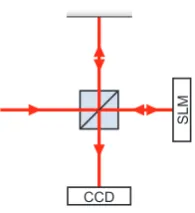
Frumker and Silberberg9make use of a Michelson interferometer (Fig. 3.1). The SLM area

is divided into two parts: one half is left unchanged while the other half is scanned through the

phase range. By analysing the resulting interference pattern with a camera, the input/phase

relation can be retrieved.

A similar method is suggested by Holoeye in the documentation of the SLM. Using an

opaque plate with two slits, they split up the beam into two distinct beams as in Fig. 3.2. These

two beams are reflected off the SLM and focussed onto one spot where an interference

pat-tern can be observed with a camera. Since the two beams are incident on different halves of

(25)

Section 3.2: Calibration methods

19

Figure 3.2: Interference of two parallel beams. The lens overlaps the two beams on the CCD.

SLM

45°

Polarizer

CCD

Figure 3.3: Calibration setup using a polarizer to convert phase modulation into amplitude modulation.

SLM

Grating CCD

Figure 3.4: Calibration setup using a transmissive grating to split the beam. On the CCD interference fringes can be seen.

phase delay is applied to one of the beams, the interference fringes will shift. This shift is a

good measure of the phase delay and thus directly related to the driving voltage. The main

advantage of this method over the setup of Frumker and Silberberg, is the simple alignment.

Furthermore, Frumker and Silberberg use a beam splitter which can give unwanted reflections

and additional interference effects that complicate measuring the movement of the fringes.

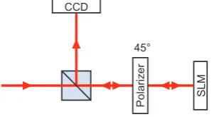
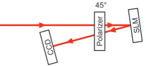
Vaughan7gives two alternative methods. In the first method, a polarizer is placed before

the SLM at 45◦_{(Fig. 3.3). The LCD is birefringent and a phase change will only be applied}

to one polarisation; the polarisation will thus change as a function of the input. By passing

the modulated beam back through the polarizer, the amplitude is modulated. The amplitude

change can be observed with a camera, and the desired relation can be retrieved.

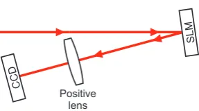
The second method used by Vaughan makes use of a (transmissive) grating (Fig. 3.4). A

monochromatic beam is split into two beams using a grating in such a way that the two beams

(26)

20

Figure 3.5: Calibration using the far field diffraction pattern of simple phase masks. The lens applies the Fourier transform to get the far field diffraction.

beams, the interference pattern of the returning beams is changed. This is essentially similar

to the Michelson interferometer, but has only one beam that has to be aligned. This is offset

by the need for a proper grating. The method proposed by Holoeye is a simplification of this

scheme. In that setup the two beams are not collinear as in the Vaughan setup, but the lack of

a prism greatly simplifies the implementation.

A final method by Chimento13 uses the field diffraction pattern (Fig. 3.5). The

far-field diffraction pattern for simple phase plates can be solved algebraically, and the measured

diffraction can thus be readily compared. Chimento uses a Heaviside function as a phase

pat-tern: a jump in phase across the middle of the SLM with a flat (but different) phase on both

halves. This is actually the same phase pattern as used in the aforementioned setups, but with

a better name. In this configuration, the relation between voltage and phase can be found by

analysing the heights and depth of the two peaks and one trough in the far field diffraction

pattern associated with the Heaviside function. The setup does require good alignment of the

beam on the centre of the phase mask, but this has the advantage of having a well aligned

beam for subsequent experiments.

The Michelson interferometer of Frumker and Silberberg; and the setup of Vaughan using

the polarizer were primarily considered for calibration of our SLM. Eventually, the method

suggested by Holoeye proved to give better results with a simpler setup. The method used by

Chimento was found later and not applied to our SLM.

There is most likely a dependence of the SLM input to phase shift correlation on the

in-coming light’s wavelength. When broadband pulses are shaped, this correlation has to be

re-established as is done in Section 4.4.

3.3 Calibration results

Initially, a simplified version of the polarisation setup of Vaughan (Fig. 3.6) was constructed to

(27)

Section 3.3: Calibration results

21

45°

SLM

Polarizer

C C D

Figure 3.6: Simplified setup with a polarizer to allow amplitude modulation. The beam is passed twice through a polarizer at 45◦while undergoing a change in polarisation on the SLM that depends on the applied phase delay. On the second pass through the polarizer, the polarisation modulation is converted into amplitude modulation.

Figure 3.7: Intensity plot of measured (left) and calculated (right) near field diffraction pattern for a phase mask with one horizontal bar of varying phase delay. The horizontal axis gives the phase delay as the input value for the SLM; the vertical axis is a cross section of the CCD.

With the polarizer in place, a checkerboard pattern was applied to the SLM with varying

sizes of the squares. The resulting intensity distributions differed greatly from the expected

patterns. For specific checkerboard sizes and phase delays the unshaped parts of the beam

would also display some amplitude modulation. To simplify the setup, only a single vertical

band of light was given a phase delay. On the camera, this again caused variations in intensity

over a much larger region of the beam. A numerical analysis of the near field diffraction offered

the explanation as can be seen in Fig. 3.7. The large distance between the SLM and the detector

(28)

22

Figure 3.8: Measured intensity for varying phase delays using a polarizer at 45◦as in Fig. 3.6. The SLM input is defined by the green colour value of the pixels sent to the SLM.

phase steps in the checkerboard pattern. This also explains the observed intensity variation in

the unshaped parts of the checkerboard patterns.

There is one important feature in Fig. 3.7 that should be recognized. There is a slight

cur-vature in the lobes of the measured intensity plot which is not present in the simulations. This

curvature is caused by the non-linear calibration of the SLM. Ideally, a linear increase in input

value (horizontal axis) leads to a linear increase of the phase delay. In reality, this relationship

is more complicated and it is precisely this relation that we are trying to determine in this part

of the project.

Moving the detector closer to the SLM reduces the extent of the diffraction pattern as the

Fraunhofer limit is approached:

R_>a 2

λ ≈30 cm, (3.1)

whereinRthe distance to an aperture with widtha. However, for complicated phase masks

with small features (ain Eq. 3.1), the effects are still noticeable.

By averaging over many measurements, it can also suffice to apply a phase delay to the

whole SLM and thus the whole laser beam. This does mean that we cannot normalise the

intensity with an unmodulated beam. Since the near field diffraction will induce intensity

fluctuations in the unmodulated beam anyway, this is a small price to pay. The laser intensity

has also proven to be sufficiently constant across the duration of the experiments to do away

with this normalisation.

The summed intensity on the CCD as a function of the SLM input is given in Fig. 3.8. On the

(29)

non-Section 3.3: Calibration results

23

linearity. However, two odd features stand out: the intensity initially rises for an increasing

phase delay and at high input values there are some jumps in intensity. We will at first ignore

these oddities and attempt to map this curve to a proper sinusoid with suitable amplitudes

and attenuation. After all, the expected plot of intensity as a function of the phase delay is a

neat sinusoid. A short explanation follows, referencing the elements of the setup as shown in

Fig. 3.6.

After the light passes the polarizer for the first time, it will have a polarisation direction

~r. We can describe this beam as a sinusoid with an amplitudeAi n and split it into two parts

with orthogonal polarisations, of which only one will be shaped by the birefringent SLM. For

simplicity, we will assume a polarisation angle of 45◦.

Ai nsin (

Here, the senkrecht polarisation direction~s(with amplitudeAs) is the polarisation

perpendic-ular to the optical table. It is this polarisation that is shaped by the SLM. The other polarisation

directionp~(with amplitudeAp) is parallel with respect to the optical table and reflected by the

SLM without modulation. Upon reflection off the SLM, a phase shiftφis imparted on the

par-allel part of the beam, leaving us with two sinusoids that have different amplitudes and a phase

shift.

Now we have an elliptically polarized beam that goes back through the polarizer at 45◦. If we

still consider the two beams separately, then the beams after polarisation are described by the

following equation.

(30)

inte-24

Figure 3.9: Calibration curves for the phase delay as a function of input level. The blue curve was obtained using amplitude modulation; the red curve is obtained using an interference pattern.

grate these sinusoids.

Apparently, all we are left with is a cosine with an offset and amplitude. For the case of a

polarizer at 45◦we haveA=B=12π, but Eq. 3.5 actually holds for all polarizer directions. For

a polarisation angleα, Eq. 3.5 becomes:

I₌

Figure 3.8 should thus be mapped to a cosine, albeit with a phase shift to compensate for

the initially rising intensity. If this is done correctly, then Fig. 3.9 is found. There are three

jumps discernable in this curve — most notably at an input of 180 — exactly there where

the measured intensity has its maxima and minimum. The accuracy with which two cosines

can be mapped around their maxima or minima is of course relatively small and as such this

method is restricted in its accuracy, at least for a part of the input values.

The initial rise of the intensity and the jumps at high input values have not yet been

ex-plained. The rise in intensity is probably caused by an inherent birefringence of the SLM.

The parallel polarisation will then always be given a phase delay compared to the orthogonal

(31)

Section 3.3: Calibration results

25

Figure 3.10: Default and new gamma curve for a 5:5 bitplane configuration.

difference and cause the intensity to rise. The jumps in intensity at higher input values can,

however, not be easily explained. They do appear to be reproducible across measurements,

but are probably caused by alignment issues as later experiments with different setups did not

exhibit this phenomenon.

Since the calibration of the SLM is limited in accuracy when using amplitude modulation,

the alternative method as suggested by Holoeye (Fig. 3.2) has also been tried. A double slit was

custom made from a business card and the resulting interference pattern was imaged onto

the CCD via two lenses. The second lens served to enlarge the image for better analysis. Half

of the SLM was kept at a fixed input level of 0, while the other half was scanned across the

256 different shaping levels. The shifts of the interference peaks were recorded and from this

the phase shift — measured in radians — was derived. The resulting relation between input

level and phase delay is compared with the amplitude modulation in Fig. 3.9. A more detailed

explanation of this calibration technique is given in Appendix B.

When the relation between SLM input level and phase delay has been determined, the SLM

software can be updated with an improvedgamma curve. The gamma curve is the internal

look up table of the SLM which converts the input of the user to the appropriate voltage for the

liquid crystal. Ideally, a linear increase in SLM input leads to a linear increase in phase delay.

Adjusting the gamma curve based on the calibration experiments explained above, allows us

to obtain this linear input-phase relation.

For the current configuration (see Section 3.4), there are 192 discrete voltage levels

avail-able to drive the SLM. We thus have to map 256 (8 bit) input values to 192 voltages in such

(32)

de-26

Figure 3.11: Measured phase delay as a function of input level for a 5:5 bitplane configuration using the default gamma curve (blue) and the optimized gamma curve (red).

Figure 3.12: Observed interference pattern shift for increasing phase delays. Shift with default gamma curve (left) and optimized gamma curve (right). With the new gamma curve a linear relation between the SLM input and the associated retardance is obtained.

fault gamma curve is shown in Fig. 3.10. With this curve loaded in the SLM, we obtain the

phase delays as in Fig. 3.11. Using the default gamma and the associated phase delays, we can

find a new gamma curve that should give a linear phase delay. The observed interference

pat-terns before and after the calibration are shown in Fig. 3.12 and it is clear that this calibration

method allows us to obtain a linear relation between the input values and the resulting phase

delay.

3.4 Bitplane configuration

After obtaining the improved gamma curve, a very simple helical phase mask was applied to

(33)

Section 3.5: Spatial shaping results

27

Figure 3.13: Laguerre-Gaussian beam profile showing radial asymmetry.

was clearly visible, a strong vibration was also present in the beam profile. This vibration was

not caused by mechanical vibrations in the system, or by instabilities in the laser. Holoeye

confirmed that this flickering is caused by the SLM, and they consider it normal behaviour:

“Due to the limited viscosity of the LC molecules these molecules flicker a little bit around

the mean value.” They suggested reconfiguring the SLM to use a 5:5 bitplane configuration,

instead of the default 22:6 bitplane configuration.

By changing the bitplane configuration, the addressing frequency of the liquid crystals can

be increased. While the driving electronics only accept 60 frames per second from the

com-puter, internally they can duplicate these frames. Each frame is then sent several times to the

liquid crystals within the refresh rate of 60Hz. However, as more updates are sent to the

crys-tals each second, less information can be contained in each. As a result, some resolution is lost

in the driving voltage of the SLM. With a 22:6 bitplane configuration 1472 voltage levels are

ac-cessible (through 256 input levels), while with a 5:5 bitplane configuration only 192 voltage

levels are accessible (through 256 input levels).

After setting the bitplane configuration to 5:5 some reduction of the flickering was found.

Even with the 5:5 bitplane configuration, a strong temporal dependence of the phase shaping

effectiveness is found. Frumker and Silberberg report a similar modulation with a

characteris-tic frequency of 300 Hz.9They assign this flickering to the electronic modulation scheme and

state that this is not a physical limitation of the liquid crystals.

3.5 Spatial shaping results

Some very simple beam profiles and diffraction patterns have been created with spatial

shap-ing. The Laguerre-Gaussian beam mentioned in Section 3.4 was made by applying a helical

(34)

28

Figure 3.14: Optimisation of phase mask for a complicated target using the Gerchberg-Saxton algorithm. After only a few iterations a good approximation of the target is obtained.

point, the beam will then destructively interfere. In this way, a donut mode is created.

Apart from the jittering mentioned earlier, there is a radial asymmetry in the resulting

beam profile as can be seen in Fig. 3.13. A similar effect is observed by Chimento using a MEMS

device.13The asymmetry is not dependent on the orientation of the phase mask, and

chang-ing the position of the beam on the SLM only has a small influence on the intensities of the two

lobes but not on their positions. The asymmetry can be ascribed to the spatial deformation of

the SLM as well as the non-uniform effective phase delay discussed in Section 3.6.

More complicated beam patterns require the calculation of unintuïtive phase masks. The

Gerchberg-Saxton (GS) algorithm14gives a way of iteratively optimising a phase mask to

ap-proximate a known target image in the focal plane. For most problems a good approximation

of the target is obtained after only a few iterations, (Fig. 3.14). If strong restraints — such as

binary phase steps — are added, convergence is less good. Many alternatives to the GS

algo-rithm are available15–17, but none share its simplicity and speed. Of course, this is offset by less

noise, sharper features, and less zero-order light. In our work, the speed of the GS algorithm

was preferred over the accuracy of its alternatives. With proper optimisations, phase mask

calculations at video-rate may even be possible.

In the GS algorithm (Fig. 3.15), an initial random phase mask is applied to the known

(Gaussian) amplitude profile of the incident beam and the result is Fourier transformed to

obtain the Fraunhofer diffraction pattern at the focal plane. While the calculated phase is

maintained, the amplitude is replaced by the desired amplitude of the target image and the

inverse Fourier transform is calculated. The resulting phase is the new phase mask, and the

amplitude should be replaced with the known amplitude of the incident beam. This process

can then be repeated ad infinitum.

In principle, the GS algorithm could also be used with a feedback loop. If the far field image

— containing the actual amplitude profile as opposed to the calculated targetAd— is captured

with a camera, this can be used to approximate the additional phase shaping from the optical

(35)

Section 3.6: Effective phase delay

29

Figure 3.15: The Gerchberg-Saxton algorithm. (Ref. 14)

in the SLM itself. With this additional shaping in mind, a new phase mask can be calculated

in order to get an improved image on the camera. When this process is repeated, a noticeable

improvement can be obtained. A slight experimental complexity that has to be overcome is

the mapping of the measured beam profile to the matrices in the algorithm. In order to get

good resolution both on the SLM and in the focal plane, the desired image has to fill the whole

matrix used in the GS algorithm. This means that in the experimental setup one also gets

a very large image which could not be projected onto the available camera. Ordinarily, the

Fourier transform could be applied to a larger matrix padded with zeroes in order to obtain a

smaller image with equal resolution. However, given that the SLM already has 2 megapixels,

this makes the calculations infeasible. A better solution would be to sacrifice some resolution

in both domains and use some appropriate lenses to project the image onto the camera.

The large diffraction patterns calculated with the GS algorithm are all easily viewed with

the naked eye. The vibrations of the liquid crystals do not have a noticeable effect in that case

due to the inherent temporal filtering of the human eye.

3.6 Effective phase delay

In the specification sheet of the SLM, Holoeye discusses the optical flatness of the display. The

listed maximal deviation of the SLM surface is 3–4 waves at 633 nm. This is much larger than

the customary flatness of mirrors in the order of tens of nanometers. Since the deformation is

(36)

30

Figure 3.16: Phase mask applied to the SLM for obtaining the effective phase delay per superpixel. The light from A and B is steered off from the main bundle via a diagonal grating. At A, an additional, variable, flat phase is added on top of the sawtooth grating in order to obtain the effective phase delay of the pixels in A (bottom).

the SLM slightly out of focus. Additionally, a phase mask can be applied to the SLM that

fur-ther compensates the deformations. However, the varying thickness of the LC panel will also

influence the phase delay range. In order to analyze the variation in effective phase delay, a

novel calibration method has been developed.

Because the HEO 1080P SLM is a two dimensional display, gratings can be displayed that

can steer incident light off into higher diffraction orders. By applying such a grating to a small

part of the display, a part of the light can be diffracted onto a camera. We use this to very

selectively analyze small parts of the SLM. The effective phase delay is then determined using

the same method as in Section 3.3.

All the light is steered off vertically into a higher diffraction order, as shown in Fig. 3.16. To

two small squares of 32 by 32 pixels a different grating is applied that diffracts a part of the light

away from the main beam. By using a diagonal grating, we obtain the least interference from

the rest of the light. The applied grating has a phase range of 0 to 128 input levels. This leaves

another 127 input levels for a constant phase delay. One of the two squares is thus given an

ad-ditional variable phase delay and the resulting shift of the interference pattern is recorded with

a camera. This process is repeated for the whole SLM, subdivided into superpixels of 32 by 32

pixels. The maximal phase delay per superpixel is then plotted to give a map of the maximal

retardance as a function of position on the LC display. A characteristic plot is given in Fig. 3.17.

(37)

ad-Section 3.6: Effective phase delay

31

Figure 3.17: Maximal phase delay per superpixel as a function of position on the SLM. The variation per superpixel is up to 10% per measurement; the overall shape, however, is constant.

-6%

Figure 3.18: Fast fluctuations in the maximal phase delay of one superpixel in the middle of the SLM. The vibrations are undersampled due to the response time of the CCD.

ditional thickening is observed at the left side of the SLM. The measured delay differences also

correspond well with the 1.8–2.4µm maximal thickness difference reported by Holoeye. Given

a common LC thickness of roughly 10µm, a 2µm thickness difference results in a maximal

phase delay bandwidth of 0.75π, similar to the results shown in Fig. 3.17.

Despite long integration times of 30 ms, a strong time dependence was observed with

max-imal variations of 10%. First of all, there are very fast fluctuations as in Fig. 3.18, where the

maximal phase delay for one superpixel is shown as a function of time. These variations have

(38)

32

Figure 3.19: Slow fluctuations of the maximal phase delay of one superpixel in the middle of the SLM.

-8%

Figure 3.20: Difference in shaping effectiveness between two consecutive measurements. Fig. 3.17 gives one of the two original measurement series.

(in the measurements these vibrations were undersampled due to the finite response time of

the CCD). Apart from the high frequency vibrations, a much slower time dependence is also

observed. By increasing the integration time of the CCD, these variations can be easily

ob-served. Fig. 3.19 shows the change in maximal phase delay over the space of several

min-utes. When two consecutive characterisations of the SLM are done, the influence of the long

term fluctuations becomes more apparent. Fig. 3.20 shows the difference between two

mea-surement series. The total meamea-surement time per superpixel is about 3 seconds and the time

between the two measurement series is several hours. Strong variations of up to 10% are

(39)

Section 3.6: Effective phase delay

33

is comparable between different measurements. Real pixel-by-pixel calibration is thus

unfea-sible, but a good profile can be obtained by applying a smoothing filter to the measured profile

(40)

(41)

4

Spectral shaping

With the basic calibration of the spatial light modulator described in Chapter 3, we now turn

to the spectral domain. First, the setup and alignment of a folded 4f zero dispersion pulse

compressor setup is explained, after which a quick and simple method for wavelength versus

pixel calibration is introduced. The spectral shaping capabilities of the SLM are demonstrated

using a second harmonic generation experiment.

4.1 Femtosecond laser source

A Coherent Legend Elite Ti:Sapphire laser amplifier is used to generate femtosecond pulses at

800 nm with a FWHM bandwidth of 36 nm. The amplifier is pumped with a tuneable

Coher-ent Micra Ti:Sapphire laser, which in turn is pumped by an integrated Verdi laser. The pulses

emerge with a power of 3 W and a repetition rate of 5 kHz. Since the amplifier is needed to

power a Coherent OPerA Solo Optical Parametric Amplifier, only a part of the 3 W is sent into

the shaper setup. As the maximum permissible power for the SLM is not known to us or the

(42)

36

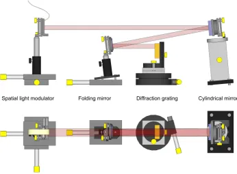
Chapter 4: Spectral shaping

Figure 4.1: Spectral shaping setup; the yellow control knobs are used for fine adjustment of position and rotation of the various elements in the setup.

4.2 Shaper setup

For shaping in the spectral domain, the SLM is placed in a 4f zero dispersion pulse

compres-sor.4Since the Holoeye HEO1080P is a reflective SLM, the incoming and outgoing pathways of

the shaper setup are identical.

A plan of the setup is given in Fig. 4.1. The broadband pulse is initially dispersed on a gold

coated ruled diffraction grating from Edmund Optics with 830 lp/mm and a blaze angle of 19◦

for 800 nm. After passing a folding mirror, the first order diffraction is focussed by a 25 cm

cylindrical mirror which was gold coated in-house.

The folding mirror and SLM are placed on linear stages with micrometer screws for fine

ad-justment of the distances to the cylindrical lens. A second linear stage under the SLM moves

it perpendicular to the propagation plane for alignment of the spectrum on the SLM. Both the

cylindrical mirror and the grating are affixed to AMOLF-built mounts that allow fine

(43)

Section 4.2: Shaper setup

37

4.2.1 Alignment

The alignment of the shaper setup is a multistep process which is complicated by the small

form factor of the setup as well as the — partially invisible — wavelength range of the laser

source.

First and foremost, the grating has to be aligned so that all diffraction orders are in the

same plane as the incident beam. This ensures that the first diffraction order emerges parallel

to the table from the grating.

The initial alignment steps are done in the zero order. In those instances, a mirror should

be substituted for the SLM to prevent accidental burning of pixels in the focus of the zero order.

• One after another, the grating, folding mirror, and cylindrical lens are placed into

posi-tion, ensuring that the beam always emerges straight along the same path.

• The replacement mirror is placed at the position of the SLM. The rotation of this mirror

must be such that the incoming and outgoing beams on the grating overlap

horizon-tally. This can be checked easily with an IR viewer. Vertically, some tilt has to be applied

in order to separate the two beams spatially on the grating. The distance between the

re-placement mirror and the cylindrical lens is adjusted until a collimated beam is obtained

at the output of the shaper.

• The grating is rotated to the first order. The proper rotation is obtained if a collimated

beam again emerges from the shaper and the two spots on the grating overlap.

• The mirror is replaced with the SLM and the distance between the SLM and the lens is

adjusted until a collimated outgoing beam is again obtained.

• If the pulse length can be measured with an autocorrelator, then the folding mirror

position can be adjusted by optimising for a minimal pulse length after the shaper.

After these steps, the spatial dispersion in the emerging beam must be minimized. This is

most easily done by applying a grating to the SLM such that most light is diffracted away from

the main beam, apart from narrow bands both at the far right and far left of the spectrum. By

alternating between the red and blue part of the spectrum, the precise position of the different

colours can be determined.

The vertical separation between the left and right part of the spectrum is adjusted by

(44)

38

760 770 780 790 800 810 820 830 840

In

Figure 4.2: Spectral dip observed when a 32 pixel wide grating is applied at pixel 743. By scanning a grating across the SLM, the wavelength versus pixel relation can be obtained.

compensated for by rotating the grating and SLM in unison. If the initial alignment has been

done properly, this should not be necessary.

4.3 Wavelength versus pixel calibration

To determine which colour is focussed on which pixel, the two dimensional shaping

capabili-ties of the SLM can be employed. By applying a grating in the vertical direction of the SLM, the

beam can be realigned spatially. If this grating is applied selectively to a band of a few pixels

wide, it is possible to steer off a part of thespectrumof the beam. By analyzing the resulting

spectrum, the wavelength versus pixel calibration is easily obtained.

Figure 4.2 shows a typical measurement as the grating is scanned along the LCD. After

an initial determination of the peak position, the accuracy in the wings of the spectrum is

improved by extrapolating the well-defined peak positions in the centre of the spectrum to the

less intense wings. In this way, an accurate determination of the wavelength per SLM pixel can

be determined as shown in Fig. 4.3.

4.4 Wavelength versus effective phase delay

As previously explained in Section 3.6, we can determine the maximum retardance as a

func-tion of locafunc-tion on the SLM. This allows us to determine the relafunc-tion between wavelength and

the effective maximal phase delay. For this purpose only a scan in the spectral dimension of

(45)

Section 4.4: Wavelength versus effective phase delay

39

0 200 400 600 800 1000 1200 1400 1600 1800

W

Figure 4.3: Pixel versus wavelength calibration. In the wings of the spectrum the accuracy of the calibration is reduced due to the low intensities.

0

750 770 790 810 830 850

In

Figure 4.4: Retardance (blue dots) as a function of wavelength for maximal SLM input. A linear fit (green line) is drawn through the points where the intensity (red line) was sufficiently high. In the wings of the spectrum, the error in the maximum retardance is too great for an accurate fit.

By determining the effective phase delay, we can also verify the SLM input vs. phase delay

relation found in Section 3.3. For all wavelengths of the laser system used, we still find a linear

SLM input vs. phase relation. There is thus no need to create look up tables to convert a desired

phase delay to the appropriate SLM input for each wavelength, but the single gamma curve

within the SLM suffices.

Figure 4.4 shows the maximum retardance as a function of wavelength. The input

spec-trum is overlaid for comparison. In the wings of the specspec-trum the observed interference

(46)

40

of the measurements.

The large spread in the measured effective phase delays can be ascribed to the temporal

variations described in Section 3.6. Nevertheless, a linear fit can be made through the points

where the maximum retardance could be determined with high confidence. A near constant

effective phase delay is found across the whole spectrum of the femtosecond pulses. Since the

temporal fluctuations of the SLM are much larger than the influence of the wavelength on the

effective phase delay, it is deemed unnecessary to compensate for this minor change in later

experiments.

The results in Fig. 4.4 are not compensated for the spatial distortion found in Section 3.6.

Apparently, the spatial distortion of the SLM and the wavelength dependent refractive index of

the liquid crystals, combined with the alignment of the SLM in the 4f configuration, result in

a near constant effective phase delay across the whole SLM. In later experiments with spectral

shaping we can thus also forego compensating for the spatial inhomogeneity of the SLM.

4.5 Second harmonic generation

One of the simplest experiments that applies phase shaping of ultrashort pulses, is the

opti-misation of second harmonic generation (SHG) in a non-linear crystal. In such a crystal, the

incoming pulses are converted into light with half the wavelength — the second harmonic

— with an efficiency that is dependent on the intensity of the pulse. SHG is aχ2process,

as in Eq. 4.1.18,19A shorter pulse of equal energy will result in higher SHG efficiency as the

peak power is greater. By optimising the SHG signal, the pulse duration is optimised to

ap-proach a transform limited pulse (the shortest possible pulse). In the spectral representation

this corresponds to a flat phase profile across the spectrum.

~

P(t)=²0¡χ1~E(t)+χ2~E2(t)+χ3E~3(t)+. . .¢ (4.1)

A detailed description of the algorithm used to find the flat phase profile is given in

Chap-ter 6. In short, the SHG signal of a random sample of phase profiles is measured, afChap-ter which

a computer algorithm suggests a new set of phase profiles of which the SHG signals are then

again measured. With each loop through the optimisation — one generation — the SHG signal

slightly improves, and the optimisation is terminated after a fixed number of generations, or

when a stable phase mask is obtained.

(47)

pro-Section 4.6: SHG optimisation setup

41

Figure 4.5: Setup for measuring SHG. Two photodiodes measure the SHG signal as well as a reference signal from the reflection from the focussing lens.

file that compensates best for phase distortions in the input pulse as well as for the effects of

elements in the beam path such as dispersion in lenses. Important to note is that distortions

occurring after the shaper are also compensated for.

SHG optimisation occurs purely in the spectral domain and thus does not make use of

the two dimensional characteristic of the SLM. If the second (spatial) direction would also be

optimised, the spatial and spectral optimisation could not be decoupled and no information

can be extracted from the optimisation. Moreover, any spatial optimisation would be purely

related to alignment of the SHG experiment, while the spectral optimisation gives insight into

the pulse characteristics. Most other experiments call for transform limited pulses which is the

main motivation to do an SHG optimisation experiment. Optimising the spatial dimension

may result in higher SHG efficiency, but does not improve the beam characteristics. Most

probably, a spatial optimisation would be restricted to improved focussing of the beam onto

the non-linear crystal.

4.6 SHG optimisation setup

After being shaped, the beam is focussed onto a thin Beta Barium Borate (BBO) crystal of

25µm with a 3.5 cm lens as in Fig. 4.5. The SHG signal is filtered with a bandpass filter,

de-tected with a photodiode and enhanced via a transimpedance amplifier. A second photodiode

measures the reflectance from the lens as a reference.

The measured second harmonic signal is divided by the reference to compensate for

fluc-tuations in both laser- and shaper stability. The result of this is normalized with the SHG

ob-tained with no phase mask applied to the SLM. The resulting amplification factor is used as

(48)

42

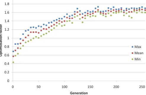
Figure 4.6: Best, mean, and worst fitness values per generation of a characteristic SHG optimisation run. This optimisation took two hours to complete with about 10,000 phase masks evaluated.

0

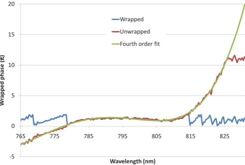
765 775 785 795 805 815 825

U

Figure 4.7: Best phase mask using a photodiode to measure SHG signal. The wrapped phase (blue line, left axis) can be unwrapped to obtain the red line (right axis). The pha