Improved Simultaneous Estimation of Location and System Reliability via Shrinkage Ideas

(1)

University of South Carolina

Scholar Commons

Theses and Dissertations

2017

Improved Simultaneous Estimation of Location

and System Reliability via Shrinkage Ideas

Beidi Qiang

University of South Carolina

Follow this and additional works at:https://scholarcommons.sc.edu/etd Part of theStatistics and Probability Commons

This Open Access Dissertation is brought to you by Scholar Commons. It has been accepted for inclusion in Theses and Dissertations by an authorized administrator of Scholar Commons. For more information, please [email protected].

Recommended Citation

(2)

Improved Simultaneous Estimation of Location and System Reliability Via Shrinkage Ideas

by

Beidi Qiang

Bachelor of Science Denison University, 2012

Submitted in Partial Fulfillment of the Requirements

for the Degree of Doctor of Philosophy in

Statistics

College of Arts and Sciences

University of South Carolina

2017

Accepted by:

Edsel Pena, Major Professor

Lianming Wang, Committee Member

Paramita Chakraborty, Committee Member

Gabriel Terejanu, Committee Member

(3)

Acknowledgments

I acknowledge NIH Grant P30GM103336-01A1 and NIH R01CA154731. I would like

to show my gratitude to Professor J. Lynch, and graduate students P. Liu, S. Shen,

(4)

Abstract

In decision theory, when several parameters need to be estimated simultaneously,

many standard estimators can be improved, in terms of a combined loss function.

The problem of finding such estimators has been well studied in the literature, but

mostly under parametric settings, which is inappropriate for heavy-tailed

distribu-tions. In the first part of this dissertation, a robust simultaneous estimator of

loca-tion is proposed using the shrinkage idea. A nonparametric Bayesian estimator is

also discussed as an alternative. The proposed estimators do not assume a specific

parametric distribution and they do not require the existence of finite moments. The

performance of proposed estimators are examined in simulation studies and financial

data applications. In the second part, we extend the idea of simultaneous estimation

in the context of estimating system reliability when component data are observed.

We propose an improved estimator of system reliability by using shrinkage

estima-tors for each of the component reliabilities and then utilize the structure function to

combine these estimators to obtain the system reliability estimator. The approach

is general since the shrinkage is not on the estimated parameters of component

reli-ability functions, but is instead on the estimated component hazard functions, and

is therefore extendable to the nonparametric setting. The details in nonparametric

setting are discussed in a later chapter. Simulation results are presented to examine

(5)

List of Tables

Table 3.1 Simulated Estimators Under Normal Distributions. k=3 and

n=5. Confidence intervals are indicated in parentheses. . . 15

Table 3.2 Simulated Estimators Under Laplace Distributions. k=3 and

n=5. Confidence intervals are indicated in parentheses. . . 15

Table 3.3 Simulated MSE of Estimators Under Different Distributions. These are based on 1000 simulation replications, k=10 and n=15.

Standard errors are indicated in parentheses. . . 17

Table 3.4 Relative Efficiency (in %) of the Estimators Under Different Dis-tributions. The relative efficiency is calculated with respect to

the sample median. . . 17

Table 3.5 Daily Stock Return of AAPL, AXP, BA, CAT and CSCO for

the First 10 Consecutive Trading Days Starting from January 3rd. 19

Table 3.6 Prediction MSEs of Different Location Estimators Using Daily Dow Jones Stock Return Data. Standard errors are indicated in

parentheses. . . 20

Table 4.1 Average Losses of the Estimators in Series and Parallel Systems under Exponential Lifetime Distribution. These are based on 1000 simulation replications. The systems had 10 components, and the sample size for each replication was 10. Also indicated

are the average values of the estimated shrinkage coefficientc. . . . 39

Table 4.2 Average Losses of the Estimators in Series and Parallel Systems under Weibull Lifetime Distribution. These are based on 1000 simulation replications. The systems had 10 components, and the sample size for each replication was 10. Also indicated are

(8)

Table 5.1 Average Losses of the Nonparametric Estimators in Series and Parallel Systems under Exponential Lifetime Distribution. These are based on 1000 simulation replications. The systems had 5 components, and the sample size for each replication was 15. Also indicated are the average values of the estimated shrinkage

(9)

List of Figures

Figure 3.1 The Effect of Shrinkage v.s. Sample Size. Simulation based on 1000 Replications, p=10. The relative efficiency is calculated

with respect to the sample median. . . 18

Figure 3.2 Histogram and QQ plot of Apple Stock Returns for 2683 Con-secutive Business Days, from January 2005 to August, 2015.

The returns seem to follow a heavy-tailed distribution. . . 20

Figure 4.1 System reliability functions for the series, parallel, series-parallel, and bridge systems when the components have common unit ex-ponential lifetimes and there are 5 components in the series and

parallel systems. . . 26

Figure 4.2 Estimated and True System Reliability Functions Over Time for a Series System with 10 components. The estimators are the ML based on component data and the improved estimator

based on a sample of size 10 systems. . . 38

Figure 4.3 Estimated and True System Reliability Functions Over Time for a Parallel System with 10 components. The estimators are the ML based on component data and the improved estimator

based on a sample of size 10. . . 39

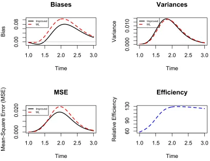
Figure 4.4 Comparing Performances of the Component-Data Based Esti-mators at Different Values of t for a 10-Component Parallel System. 1000 Replications we used, with each replication

hav-ing a sample size of 10. . . 41

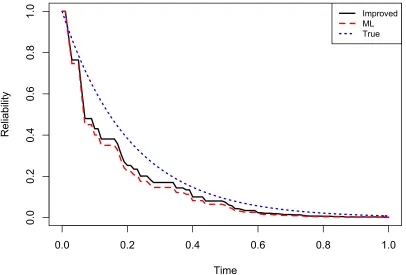
Figure 5.1 Estimated and True System Reliability Functions Over Time for a Series System with 5 components. The estimators are the nonparametric ML based on component data and the improved

(10)

Figure 5.2 Estimated and True System Reliability Functions Over Time for a Parallel System with 5 components. The estimators are the nonparametric ML based on component data and the improved

(11)

Chapter 1 Introduction

In decision theory, when several parameters need to be estimated simultaneously,

many standard estimators can be improved under a combined loss function, by a

combined estimator. The improvement of using combined information is observed,

even when using independent data to estimate those parameters. One example that

uses the idea of simultaneous estimation explicitly is the JamStein shrinkage

es-timator (13). As a biased eses-timator of the mean of Gaussian random vectors, the

James-Stein estimator dominates the standard least squares estimators in terms of

total mean squared error (MSE), when three or more parameters are estimated

simul-taneously. A lot of research has been done focusing on shrinkage estimators and the

problem of simultaneous estimators which dominate the usual maximum likelihood

estimators (MLEs) has been well studied.

One extension presented in this work is the idea of developing a more robust

shrinkage estimator under nonparametric assumptions. In the literature, most

ex-isting James-Stein type shrinkage estimators are developed under the assumption of

multivariate normal distribution. Some studies relaxed the normal assumption, but

still require the existence of finite moments. However, these assumptions may not

always be realistic when heavy-tailed data is observed. To extend the idea, a more

robust estimator based on the sample median is proposed, which does not assume

a specific parametric distribution nor requires the existence of finite moments. An

alternative estimator is also developed using nonparametric Bayesian approach. The

(12)

sim-ulation studies and empirical data analysis. The proposed estimator is expected to

outperform the usual ML estimates in heavy-tailed distributions especially in "large

p, smalln" settings.

Another natural extension is to apply the idea of simultaneous estimation to

failure time analysis, notably survival analysis and reliability, especially estimating

the reliability of a coherent system using lifetime data from its components. When

component-level data are available, the traditional way of estimating system reliability

is to find component level MLEs and then utilize these MLEs according to the system

structure to obtain an estimator of the system reliability. We propose an improved

estimator of system reliability under an invariant global loss function. Shrinkage type

estimators for each of the components reliability functions are obtained first and then

these estimators are combined according to the system structure function to obtain an

improved estimator of the system reliability. The approach is general since the

shrink-age is not on the estimated component reliability function parameters but is instead

on the estimated components hazard functions, and are therefore extendable to the

setting where the components reliability functions are specified non-parametrically.

The performances of different estimators will be compared though simulation studies.

The proposed estimator is expected to perform better under the given loss function,

as compared to the MLEs.

The rest of the dissertation is organized as follow. In Chapter 2 , the James-Stein

estimator and its extensions and applications are reviewed. The ideas and results

of extending the simultaneous estimation idea to nonparametric setting is discussed

in Chapter 3. In Chapters 4 and 5 , the shrinkage estimation method is applied to

the estimation of system reliability. Some properties of the estimator and simulation

analysis are presented. Ideas for future studies, improvements, and extensions are

(13)

Chapter 2 Some Review and Motivation

2.1 The Decision Theory Framework

A decision problem has the following elements:

(Θ,A,X,F ={F(·|θ),θ ∈Θ}, L,D)

Here Θ is the parameter space containing the possible values of some parameters θ,

which could be finite- or infinite-dimensional; A is the action space consisting of all possible actions that the decision maker could take;L: Θ×A → <is the loss function, with L(θ,a) denoting the loss incurred by choosing action a when the parameter is

θ. The observable data X takes values in the sample space X, with X, given θ, having distribution F(·|θ), which belongs to the family of distribution functions F. Non-randomized decision functions are (measurable) mappings δ : X → A, and the totality of such decision functions is the decision function space D. To assess the quality of a decision function δ∈ D, we utilize the risk function given by

R(θ, δ) = E[L(θ, δ(X)|θ)],

which is the expected loss incurred by using decision function δ when the parameter

is θ. Good decision functions are those with small risks whatever the value of θ.

In particular, a decision function δ1 is said to dominate a decision function δ2 if

for all θ ∈ Θ, R(θ, δ1) ≤ R(θ, δ2) with strict inequality for some θ ∈ Θ. In such a case the decision function δ2 is inadmissible. The statistical inference problem

of parameter point estimation falls into this decision-theoretic framework with the

(14)

2.2 On Simultaneous and Shrinkage Estimators

Simultaneous Estimation

This decision-theoretic framework carries over to simultaneous decision-making, in

particular, simultaneous estimation. Consider, for instance, the situation whereθ =

(µ1, µ2, . . . , µK) ∈ Θ = <K, the action space is A = <K, and the data observable is X = (X1, X2, . . . , XK) ∈ X = <K where the Xj’s are a normal distribution with meanµj and varianceσ2, assumed known. Xj’s are assumed to be independent, given

µj’s. For the simultaneous estimation problem, we could use the loss function given

by

L(θ,a) =||θ−a||2 ₌ K X

i=1

(µi−ai)2,(θ,a)∈Θ× A.

This loss function is referred to as quadratic loss function. The maximum likelihood

(ML) estimator of θ is δM L(X) = X, whose risk function is given by

R(θ, δM L) =E h

||θ−X||2_|_θi

=Kσ2.

Incidentally, this ML estimator is also the least-squares (LS) estimator of θ. When

K = 1 or K = 2, δM L is the best (risk-wise) estimator of θ.

James-Stein Shrinkage Estimation

James and Stein (13) demonstrated that there is a better estimator ofθthanδM L(X) =

X, when 3 or more parameters are estimated simultaneously. An estimator that

dom-inates the ML estimator is their so-called shrinkage estimator of θ, given by

δJ S(X) = θb_{J S} = "

1− (K −2)σ

2

kXk2 #

X.

More generally, ifX= (X1, . . .Xn) are IID 1×pmultivariate normal vectors with mean vectorθ, and common covariance matrixσ2_I

K, then the James-Stein estimator of θ is given by

δJ S(X) = θb_{J S} = "

1− (K −2)σ

2

nkXk2 #

(15)

where X= 1 n

Pn

j=1Xj denotes the vector of sample means.

The James-Stein shrinkage estimator is one which utilizes the combined data for

estimating each component parameter, even though the component variables are

in-dependent, to improve the simultaneous estimation of the components ofθ. It shows

that optimizing (i.e., minimizing) a global loss is not the same as optimizing

indi-vidually the loss of each component estimator. In essence, there is an advantage in

the borrowing of information from each of the component data, demonstrating that

when dealing with a combined or global loss function, it may be beneficial to borrow

information in order to improve the estimation process. Observe that the James-Stein

type of shrinkage estimator is of the form

δc(X) = ˆθc=cX,

for some c >0, which in this case is data-dependent.

An Empirical Bayes Approach

The James-Stein Shrinkage estimator can be developed using the empirical Bayes

method (9). Suppose X = (X1, . . .Xn) are IID 1×p multivariate normal vectors with mean vector θ, and common covariance matrix σ2IK. If we place a N(0, τ2IK)

prior on the vector θ, the posterior distribution ofθ is

θ|X1, . . .Xn ∼N

τ2

τ2₊_σ2_/nX,

₁

τ2 +

n σ2

−1!

.

The Bayes estimator of θ is the posterior mean, which is given by

ˆ

θBayes =

τ2

τ2₊_σ2_/nX. (2.1)

The hyper parameter τ2 is then estimated from the data, which makes the

(16)

free-dom. When K ≥3,

E

"

(σ2_/n₊_τ2₎

||X||2 #

= 1

K−2, and τ2 is estimated by

ˆ

τ2 = ||X|| 2

K−2 −

σ2

n .

The James-Stein Estimator is then recovered when replacingτ2 by ˆτ2 in (2.1).

Motivation

In the literature, some generalizations of James-Stein type shrinkage estimators were

developed, but most existing methods use the assumption of normal distribution.

However, in "large p, small n" problems, the sample covariance matrix is usually

singular, and thus traditional shrinkage methods cannot be applied. Wang et al.

(28) proposed a shrinkage estimator for population mean under quadratic loss with

unknown covariance matrices. Although no specific distribution is assumed, their

non-parametric shrinkage estimator is based on the sample mean and does require the

distribution to have finite moments. This assumption can be unrealistic when the data

follow some heavy-tailed distribution, such as the Cauchy. Therefore, more robust

shrinkage estimators based on nonparametric assumptions are developed through the

shrinkage idea and the Bayesian approach in Chapter 2.

The application of shrinkage estimation in survival analysis has also been partly

addressed in the literature. In (27) three versions of shrinkage estimators under

expo-nential lifetimes were examined. Later, in (24) shrinkage estimators under the LINEX

loss function in the situation with exponential lifetime censored data were presented.

The shrinkage estimation of the reliability function for other lifetime distributions

were also studied in (6) and (23). The extension to the estimation of the system

reliability has also been discussed under certain system structures and lifetime

distri-butions, see, for instance, (21; 22). Instead of developing estimators under a specific

(17)

estimation is extended to general system structures and lifetime models. Improved

estimators of component reliability functions are developed under an invariant global

loss function. The improved estimators are developed under a general framework,

(18)

Chapter 3 Robust Simultaneous Estimator of Location

3.1 Idea and Motivation of Estimator

To relax the normality assumption and provide a more robust estimator in

simulta-neous estimation, we extend the shrinkage idea into nonparametric settings, where

heavy-tailed distributions are allowed. The nonparametric shrinkage estimator is

then applied to stock return data, since such data is believed to have heavy-tailed

properties based on empirical evidence.

Consider i.i.d 1×K vectors X1, . . .Xn that satisfy

Xi =µ+i,Xj ∈ <K,i = (i1,· · · , iK),

where ij’s are identically and independently distributed and follow some symmetric

distribution Fj that is centered at 0, for i = 1, . . . , n, j = 1, . . . , K. Fj’s are

un-known. Consider the simultaneous estimation problem of estimating of the location

parameters µj’s, with respect to the quadratic loss function

L(µ,µb) =||µb −µ|| 2_,

where µ= (µ1, µ2, ..., µK).

A common nonparametric approach is to estimate the location parameters by the

sample medians. But using the idea of simultaneous estimation, some improvement

can be achieved, in terms of the combined MSE. Consider estimatingµj by a shrinkage

of the sample median, Xf_j, i.e.

b

(19)

When sample size n is odd, Xf_j ≡X₍n+1

2 )j. The goal is to find the optimal c in terms

of the combined expected loss function. However, this optimal coefficient c∗ may

depend on the unknown parameters. Thus an estimator ofc∗ will be used in practice.

The James-Stein shrinkage estimator can be viewed as an empirical Bayes

esti-mator when putting a normal prior on the parameters µ. So we also seek a Bayes

approach to develop a robust shrinkage estimator. A Dirichlet process prior is used

given the nonparametric setting.

3.2 Evaluating the Estimators

To find the optimal amount of shrinkage, the risk or expected lossE[L(µb)] =E[||µb−

µ||2_{] is minimized with respect to}_c_.

R(µ,µb(c)) = E[L(µ,µb(c))]

= K X

j=1

E[cXf_j−µ_j]2

= c2

K X

j=1

var(Xf_j) + (c−1)2||µ||2,

where var(Xf_j) denotes the variance of the sample median in sample j. Thus the

optimal shrinkage coefficient cis given by

c∗ = 1−

PK

j=1var(Xfj)

||µ||2₊PK

j=1var(Xfj)

<1.

The corresponding risk of ˆµ∗ is then

E(L(µ,µˆ∗)) = (c∗)2 p X

j=1

var(Xf_j) + (1−c∗)2||µ||2.

Notice the sample median, Xf_j, has an asymptotic normal distribution with mean θ_j

and variance [4nfj(θj)2]−1. Thus, var(Xf_j) goes to 0 as sample size increases, and thus

the shrinkage coefficient c∗ converges to 1 when sample size converges to infinity, i.e.

(20)

3.3 Estimating the Shrinkage Coefficient c∗

In practice, in the expression ofc∗, the true location parameters and the variances of

the sample medians are unknown since theFj’s are unknown and need to be estimated

based on the observed data. In the nonparametric setting, the sample median of Xj

is used as a robust estimator of µj. Thus ||µ||2 is estimated by

||µ||2 _≈ f

X₁2+Xf₂2+· · ·+Xf_K2

To estimate the variance of the sample median nonparametrically, we adopt the

method proposed by Maritz and Jarrett (19). Consider the case when the sample

size is odd, i.e. n = 2m+ 1. Some modifications are needed when the sample size

is even, but follows the same idea. The moments of the sample median are given by

the following equation,

E[Xfk] =

(2m+ 1)! (m!)2

Z ∞

−∞

xk[F(x)(1−F(x))]mf(x)dx.

Substitute y=F(x) to get

E[Xfk] =

(2m+ 1)! (m!)2

Z 1

0

[F−1(y)]k[y(1−y)]mdy.

The inverse of the distribution function, F−1(x), can be estimated piece by piece by

the observed order statistics. Thus,

E[Xfk]≈ n X i=1 h X(i) ik Wi

where X(i) is the ith observed order statistics, and

Wi =

(2m+ 1)! (m!)2

Z i/n

(i−1)/n[y(1−y)] m

dy.

Combining the above results, the estimated variance of the sample median is then

given by

\

var(Xf_j)≡V_j = n X i=1 h X(i)j i2

Wi−

hXn

i=1

X(i)jWi

i2

(21)

where X(i)j is the ith order statistic in sample j.

As proved by Maritz and Jarrett (19), Vj is a consistent estimator of var(Xf_j)

when var(Xf_j) is finite. However, E(V_j) may not exist when considering long-tailed

distribution, such as Cauchy. Under Cauchy distributions, the second-order moments

of the four extreme order statisticsX(1),X(2),X(n−1), andX(n)are not finite, and thus

the expectation of V does not exist. In order to obtain a finite E(V) it is necessary

to use Winsorized estimate which does not involve the four extreme order statistics.

Winsorized estimate is obtained by replacing the smallest l order statistics by the

(l+ 1)th order statistic and replace the largestlorder statistics by the (n−l)th order statistic.

Finally, the estimated c∗ is in the form

ˆ

c∗ = 1−

PK

j=1Vj

Pp

j=1Xf_j2+Pp_j=1V_j

<1.

3.4 The Nonparametric Empirical Bayesian Approach

Since the James-Stein shrinkage estimator can be developed through empirical Bayes

approach, we seek an analog in the nonparametric setting by assuming a Dirichlet

process prior on the distribution of Xj, j = 1,· · · , K. The definitions of Dirichlet distribution and Dirichlet process are given below and more details are provided in

(11).

Definition 3.1. Assume Z1,· · · , Zk are independent random variables, with Zj ∼

Gamma(αj,1). Let Yj =Zj/Pki=1Zi. Then (Y1,· · · , Yk) follows a Dirichlet distribu-tion with parameters (α1,· · · , αk), denoted by (Y1,· · · , Yk)∼ D(α1,· · · , αk).

Given the definition of a Dirichlet distribution, one can show that if (Y1,· · ·, Yk)∼

(22)

variable withP r(X =j|Y1,· · · , Yk) = Yj, then the distribution of (Y1,· · · , Yk)|X =j is also Dirichlet, with parameters (α1,· · · , αj+ 1,· · · , αk).

Definition 3.2. Letα be a nonnegative, finitely additive, finite measure on (X,A).

P is a Dirichlet Process on (X,A) with parameter α, if for all k = 1,2,· · · and for all measurable partitions (B1,· · · , Bk) of X,

(P(B1),· · · , P(Bk))∼ D(α(B1),· · · , α(Bk)).

The following theorem provides a way of updating prior beliefs in response to

observed data using Bayes’ rule.

Theorem 3.3. IfP is a Dirichlet Process on(X,A)with parameterαandX1,· · · , Xn

is a sample from P, then the posterior P|(X1,· · · , Xn) is a Dirichlet Process on (X,A) with parameter α+Pn

i=1δXi, where δXi(A) =I(Xi ∈A) (11).

Consider i.i.d 1×K vectors X1, . . . ,Xn that satisfy Xij ∼ Fj, j = 1,2,· · ·, k,

i = 1,2,· · · , n. We put i.i.d Dirichlet Process prior on Fj, i.e. Fj ∼ Dir(α). Then according to Theorem 3.3, the posterior Fj|(X1, . . . ,Xn), is a Dirichlet process with parameter α+Pn

i=1δXij. By definition of Dirichlet process, for a measurable set B,

(Fj(B), Fj(Bc))|(X1, . . . ,Xn) ∼ D(α(B) +Pni=1I(Xij ∈ B), α(Bc) +Pni=1I(Xij ∈

Bc_{)). Therefore, we obtain an estimate of ˆ}_F

j(B), given by

ˆ

Fj(B) = E[Fj(B)|X1, . . . ,Xn] = α(B) +

Pn

i=1I(Xij ∈B)

α(<) +n

= α(<)

α(<) +n · α(B)

α(<) +

n α(<) +n ·

1

n

n X

i=1

I(Xij ∈B)

(23)

data. To estimate α empirically, observe that

E[I(Xij ≤t)] = E{E[I(Xij ≤t)|Fj]} = E(Fj(t))

= α((−∞, t])/α(<).

As mentioned in (11), α(<) is a measure of faith in the prior and if α(<) is small compared to sample size, more weight is given to the observations. Therefore, we

take α(<) =√nk as a reasonable choice suggested in (25). Then α((−∞, t]) can be estimated empirically by

1 √ nk k X j=1 n X i=1

I(Xij ≤t). The empirical Bayes estimator ofFj is then given by

ˆ

Fj(t) =

√

nk

√

nk+n ·

1 nk k X j=1 n X i=1

I(Xij ≤t) +

n

√

nk+n ·

1

n

n X

i=1

I(Xij ≤t).

Notice that ˆFj(t) is a weighted sum of the empirical distribution based on the data

from sample j and the empirical distribution based on the data from all samples.

Thus, ˆFj(t) can be viewed as a shrinkage of the empirical distribution of sample j

towards the average empirical distribution of all samples.

The Nonparametric Bayesian Shrinkage Estimator (NBSE) of the location

param-eter is then the median of the estimated distribution, which can be found by solving

the following equation for t.

ˆ

Fj(t) =

√

nk

√

nk+n ·

1 nk k X j=1 n X i=1

I(Xij ≤t) +

n

√

nk+n ·

1

n

n X

i=1

I(Xij ≤t) = 1 2.

Since the ˆFj(t) is a step function with discontinuities at theXij’s, numerical solution

will be used but exact equality may not be obtained. We taket∗ = arg inf[Fj(t)>0.5]

(24)

3.5 Constructing Confidence Intervals

In this section, we present one approach to constructing corresponding confidence

intervals. Given the nonparametric setting and the form of the estimators, a bootstrap

approach is applicable. The steps are as follows.

1. At iteration m, randomly resample n times from the index set {1,2,· · ·n}

with replacement, where n is the size of the original data. This gives indices

Im1,· · · , Imn.

2. From each original sample j, j = 1,· · · , K, take Xmj = (XIm1j,· · · , XImnj).

TheXmj’s forms a new data with sample size equals to the original sample size.

3. Calculate the estimator of location using methods from the previous sections

based on the bootstrap data. This gives an estimate ˆµ_m = (ˆµm1,· · · ,µˆmK) of the location vector.

4. Repeat step 1 to 3 M times, save ˆµ₁,· · · ,µˆ_M.

5. At a confidence level of 100(1−α)%, the lower limit of the confidence interval for µj, j = 1,· · ·, K will be the 100(α/2)% percentile of the M estimates ˆ

µ1j,· · · ,µˆM j, and the upper limit will be the 100(1−α/2)% percentile of the M estimates.

We note that the resulting confidence intervals are with respect to the individual

parameters. However, simultaneous confidence intervals may be more appropriate in

the situation since we are estimating several location parameters simultaneously. The

simultaneous confidence intervals may be obtained using the Bonferroni Method or

(25)

3.6 Example and Numerical Illustration

To illustrate the performance of the estimators, we provide some numerical examples

under different distributions. We generated data based on normal and Laplace

dis-tributions. Under each distribution, a sample of n = 5 and K = 3 was generated.

Tables 3.1 and 3.2 present the estimates and confidence intervals for one replication,

along with the true location parameters.

Table 3.1: Simulated Estimators Under Normal Distributions. k=3 and n=5. Confi-dence intervals are indicated in parentheses.

True Parameter Sample Mean Shrinkage Median Np Bayesian

0.5 0.220 0.548 0.592

(-0.435,0.876) (-0.846,0.837) (-0.145,0.845)

1.0 0.586 0.781 0.844

(-0.066,1.240) (-0.242,1.260) (-0.556, 1.253)

1.5 1.235 1.279 1.253

(0.301,2.169) (-0.226,2.052) (-0.555, 2.040)

Table 3.2: Simulated Estimators Under Laplace Distributions. k=3 and n=5. Confi-dence intervals are indicated in parentheses.

True Paramete Sample Mean Shrinkage Median Np Bayesian

0.5 -0.028 0.464 1.101

(-1.385,1.328) ( -1.970,1.289) ( -1.033,1.296)

1.0 0.993 1.003 1.135

(0.124,1.863) (-0.374,1.260) (-0.380, 2.184)

1.5 2.689 2.398 2.358

(1.767,3.611) (0.928,3.618) ( 1.101, 3.618)

Since the results are only based on one replication, we cannot make definitive

com-parisons of the performance of the different estimators. However, from the tables, one

could see that the shrinkage estimates and their confidence intervals estimate the true

(26)

next section we present the results of simulation studies to compare the performance

of the different estimators in terms of average squared errors.

3.7 Simulated Comparisons of the Estimators

The performance of our method was examined when the true distribution is Normal,

Logistic, Laplace, and Cauchy. At each iteration, different true location parameters

were generated randomly from a standard uniform. The mean squared errors (MSEs)

are presented in Table 3.3, when K = 10, n= 11. We note that the presented MSEs

are not an estimator of the risk, since the data were generated under different true

parameters in each iteration.

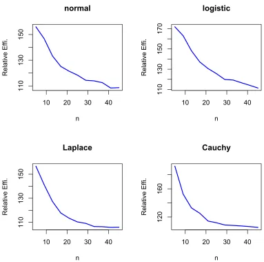
To examine the effect of shrinkage, the relative efficiency was calculated with

respect to the sample median via, for example,

RelEff = MSE(Shrinkage median)

MSE(Sample median) ×100%.

The relative efficiency presents the ratio of efficiencies of the two methods, where the

efficiency here represents the performance of an estimator in terms of the estimated

risk. The relative efficiencies are presented in Table 3.4. Based on the simulation

results, the shrinkage median estimator dominates the sample median in all cases, in

terms of mean squared error. The shrinkage median estimator is also the best when

error distribution is Laplace, and the nonparametric Bayes estimator is the best under

Logistic and Cauchy distribution. The improvement of using robust estimators over

JS estimator is most significant under the Cauchy distribution.

As mentioned earlier, the shrinkage coefficientcgoes to 1 as sample size increases.

Therefore, the improvement of using shrinkage is more significant in "large p, small

n" cases. Figure 3.1 captures the effect of shrinkage as sample size increases, under

(27)

Table 3.3: Simulated MSE of Estimators Under Different Distributions. These are based on 1000 simulation replications, k=10 and n=15. Standard errors are indicated in parentheses.

Distribution Sample JS Sample Shrinkage Np Bayesian c

Mean Median Median

Normal 0.639 0.566 0.987 0.802 0.900 0.776

(0.009) (0.008) (0.014) (0.011) (0.011) (0.0021)

Logistic 2.165 1.801 2.695 1.624 1.592 0.643

(0.030) (0.027) (0.039) (0.022) (0.021) (0.0032)

Laplace 1.383 1.102 1.006 0.756 0.761 0.722

(0.020) (0.017) (0.017) (0.012) (0.010) (0.0025)

Cauchy 2.532e+04 2.532e+04 2.099 1.300 1.262 0.612

(8.89e+03) (8.89e+03) (0.039) (0.020) (0.018) (0.0035)

Table 3.4: Relative Efficiency (in %) of the Estimators Under Different Distributions. The relative efficiency is calculated with respect to the sample median.

Distribution Sample JS Sample Shrinkage Np Bayesian

Mean Median Median

Normal 154.46 174.38 100 123.07 109.67

Logistic 124.48 149.64 100 165.95 169.28

Laplace 72.74 91.29 100 133.07 132.19

Cauchy 0.0079 0.0079 100 161.46 166.32

3.8 Application to Stock Return Data

In this section, we apply our non-parametric shrinkage method to stock return data.

Daily trading prices of 29 Dow Jones companies (we excluded Visa Inc. since its

initial public offering was in 2008) were collected in 2683 consecutive business days,

from January 3rd, 2005 to August 28th, 2015. In the context of risk management

and portfolio allocation, it is usually important to first understand the distribution

of the returns of financial assets. Thus, the variable of interest here is the daily stock

return, which is calculated as the percentage increase in the closing price from the

pervious day’s closing price, i.e. the return of day i is calculated by

returni =

Closing_i−Closing_i−1 Closingi−1

(28)

10 20 30 40 110 130 150 170 logistic n R el at ive Ef fi.

10 20 30 40

110 130 150 normal n R el at ive Ef fi.

10 20 30 40

110 130 150 Laplace n R el at ive Ef fi.

10 20 30 40

120 160 Cauchy n R el at ive Ef fi.

Figure 3.1 The Effect of Shrinkage v.s. Sample Size. Simulation based on 1000 Replications, p=10. The relative efficiency is calculated with respect to the sample median.

A portion of the data is presented in Table 3.5.

The goal is to make predictions about future returns of all stocks simultaneously

based on the return data from a previous time window. Many financial models are

developed under the assumption of normal returns. Therefore, an intuitive way is

to look at the moving averages for each stock individually. Using the idea presented

(29)

Table 3.5: Daily Stock Return of AAPL, AXP, BA, CAT and CSCO for the First 10 Consecutive Trading Days Starting from January 3rd.

AAPL AXP BA CAT CSCO

1.02705806 -1.5024064 -1.9423217 -1.1044527 -3.93374692 0.87582135 -0.9281133 1.6606681 -1.9144796 0.05388367 0.07748127 -0.5143170 -0.6494827 1.4747350 1.50780962 7.28131155 -0.7385547 -0.3367623 -0.2137263 -0.68966341 -0.41888197 0.2046050 1.3317404 -0.9209692 0.00000000 -6.38041456 -0.9281558 -0.3138500 -1.3834832 -0.42734912

1.39394534 -0.2248587 2.2038544 1.2384977 1.55579974 6.63000674 -0.6948341 -2.5221342 0.5304718 -0.79239203 0.57321328 -0.3025500 0.5530293 0.8938217 0.53247671 0.64098695 0.8156360 1.9053231 -0.8040340 -0.74152610

accordingly using the James-Stein estimator. Moreover, empirical evidences have

led to attention on the tail behavior of stock returns and it is now considered that

the returns possess heavy-tailed distributions. The Q-Q plot of the stock returns

of AAPL is presented in Figure 3.2 as an example. In heavy tailed distributions,

we expect the nonparametric shrinkage method to work better than the James-Stein

shrinkage estimator. To make prediction about stock returns on the next business

day, returns from previous 5 or 15 trading days were used as observed data. Table

3.6 presents the prediction result using different methods. The squared errors were

calculated combining all 29 stocks, and the mean and standard deviations of squared

errors were calculated, for the different methods. The shrinkage estimators perform

better in general, and the shrinkage median estimator has the smallest prediction

mean square error, followed by the nonparametric Bayes estimator. Although the

improvement is only around 1% to 2% compared with the James-Stein shrinkage

estimator, it might still be of great financial interest, given the heavy cash flow in the

(30)

Histogram of AAPL AAPL D en si ty

-10 -5 0 5 10

0.00

0.05

0.10

0.15

0.20

-3 -2 -1 0 1 2 3

-1 5 -1 0 -5 0 5 10 15

Normal Q-Q Plot

Theoretical Quantiles Sa mp le Q ua nt ile s

Figure 3.2 Histogram and QQ plot of Apple Stock Returns for 2683 Consecutive Business Days, from January 2005 to August, 2015. The returns seem to follow a heavy-tailed distribution.

Table 3.6: Prediction MSEs of Different Location Estimators Using Daily Dow Jones Stock Return Data. Standard errors are indicated in parentheses.

Lag(days) Sample JS Sample Shrinkage Np Bayesian

Mean Median Median

5 3.795 3.561 3.982 3.486 3.488

(0.208) (0.206) (0.211) (0.193) (0.198)

15 3.334 3.255 3.430 3.225 3.271

(0.170) (0.169) (0.177) (0.166) (0.173)

3.9 Summary

In this chapter, we constructed and compared the nonparametric estimators of

loca-tion using the idea of shrinkage. Confidence intervals of the localoca-tion parameter were

also provided using bootstrap approach. Based on simulation results, the shrinkage

estimator dominates the standard ones in all cases. The shrinkage median estimator

and the nonparametric Bayesian estimator are robust under unknown distributions

as compared to the James-Stein estimator. The shrinkage effect is more significant

(31)

other. We did see improvements of using the shrinkage median in the stock return

application. Though the improvements are small, it might still be of economic

inter-est.

The ultimate goal of predicting asset returns is to allocate assets in a way that

maximize the expected portfolio return as well as control the risk (20). Since the

shrinkage method provides more accurate predictions of asset returns, it might be

useful to incorporate the predictions in the portfolio allocation to achieve a higher

portfolio return.

The efficient-market hypothesis states that asset prices fully reflect all available

in-formation, which makes it impossible for investors to outperform the market through

market timing or portfolio selection. However, the application in section 3.8 shows

different prediction results when different prediction methods were used. The

shrink-age methods performs better in prediction when past stock return data are used,

which indicates the possibility of exploiting information from the past to get a better

(32)

Chapter 4 Improved Estimation of System Reliability

Through Shrinkage Idea in Parametric Settings

This portion of the dissertation will appear in Analytic Methods in Systems and

Software Testing, edited by Ruggeri, F., Kenett, R. and Faltin, F. W.

4.1 Reliability Concepts

Detailed discussions of concepts and ideas presented below are available in (3) and

(17). Consider a component with a lifetime, denoted byT, measured in some unit of

‘time’. Usually, the lifetime will be measured in literal time, but it need not always

be the case. Such a T is a non-negative random variable. The reliability function of

this component is defined via

R(t) = 1−F(t) =P r{T > t},

where F(·) is the corresponding distribution function. We assume that lifetime vari-ables are continuous. ForT, its probability density function (pdf) is

f(t) = dF(t)

dt =− dR(t)

dt .

Its hazard rate functionλ(t) is defined as

λ(t)≡lim dt↓0

1

dtP r{t≤T < t+dt|T ≥t}= f(t)

R(t),

which can be interpreted as the rate of failure of the component at timet, given that

(33)

cumulative hazard function is

Λ(t) =

Z t

0

λ(v)dv.

For a continuous lifetime T, we have the following relationships:

f(t) = λ(t) exp{−Λ(t)} and R(t) = exp{−Λ(t)} (4.1)

For a component with lifetimeT, its associated state process is{X(t) :t≥0}, where

X(t) = I{T > t} is a binary variable taking values of 1 or 0 depending on whether the component is still working (1) or failed (0) at time t. The function I(·) denotes indicator function.

Consider a system composed of K components, where this system is either in a

working (1) or failed (0) state. The functionality of a system is characterized by its

structure function

φ:{0,1}K _{→ {}₀_,₁_}_,

withφ(x1, x2,· · · , xK) denoting the state of the system when the states of the compo-nents are x= (x1, x2,· · · , xK)∈ {0,1}K. The vector xis called the component state vector. Such a system is said to be coherent if each component is relevant and the

structure function φ is nondecreasing in each argument. The ith component is

rele-vant if there exists a state vector x∈ {0,1}K _{such that} _φ₍_x_,₀

i) = 0< 1 = φ(x,1i), with the notation that (x, ai) = (x1, . . . , xi−1, ai, xi+1, . . . , xn). We will only consider

coherent systems in this chapter. Four simple examples of coherent systems are the

(i) series; (ii) parallel; (iii) three-component series-parallel; and (iv) five-component

bridge systems, whose respective structure functions are given by

φser(x1, . . . , xK) = QKi=1xi; (4.2)

φpar(x1, . . . , xK) = `Ki=1xi ≡1−QKi=1(1−xi); (4.3)

φserpar(x1, x2, x3) = x1(x2∨x3); (4.4)

(34)

The binary operator ‘∨’ means taking the maximum, i.e. a1 ∨a2 = max(a1, a2) = 1−(1−a1)(1−a2) for ai ∈ {0,1}, i= 1,2.

Let Xi, i= 1, . . . , K, be the state (at a given point in time) random variables for

the K components, and assume that they are independent. Denote bypi = Pr{Xi = 1}, i= 1, . . . , K, and let p = (p1, p2, . . . , pK) ∈[0,1]K be the components reliability vector (at a given point in time). Associated with the coherent structure function φ

is the reliability function defined via

hφ(p) = E[φ(X)] = Pr{φ(X) = 1}.

This reliability function provides the probability that the system is functioning, at

the given point in time, when the component reliabilities at this time arepi’s. For the

first three concrete systems given above, these reliability functions are, respectively:

hser(p1, . . . , pK) =QKi=1pi; (4.6)

hpar(p1, . . . , pK) = `Ki=1pi ≡1−QKi=1(1−pi); (4.7)

hserpar(p1, p2, p3) = p1[1−(1−p2)(1−p3)]; (4.8)

For the bridge structure, its reliability function at a given point in time, obtained

first by simplifying the structure function, is given by

hbr(p1, p2, p3, p4, p5) = (p1p4+p2p5+p2p3p4+p1p3p5+ 2p1p2p3p4p5)

−(p1p2p3p4+p2p3p4p5+p1p3p4p5+p1p2p3p5+p1p2p4p5). (4.9)

Of more interest, however, is viewing the system reliability function as a function of

time t. Denoting by S the lifetime of the system, we are interested in the function

RS(t) = Pr{S > t}

(35)

processes is{X(t) = (X1(t)· · · , XK(t)) :t≥0}. The system lifetime is then

S = sup{t≥0 :φ[X1(t),· · · , XK(t)] = 1}.

The component reliability functions are Ri(t) =E[Xi(t)] = Pr{Ti > t}, i= 1, . . . , K. If the component lifetimes are independent, then the system reliability function

be-comes

RS(t) =E[φ(X1(t), . . . , XK(t))] = hφ(R1(t), . . . , RK(t)). (4.10)

That is, under independent component lifetimes, to obtain the system reliability

function, we simply replace thepi’s in the reliability functionhφ(p1, . . . , pK) byRi(t)’s.

For the concrete examples of coherent systems given in (4.2–4.5), we therefore obtain:

Rser(t) =QKi=1Ri(t); (4.11)

Rpar(t) = 1−Qi=1K (1−Ri(t)); (4.12)

Rserpar(t) =R1(t)[1−(1−R2(t))(1−R3(t))]. (4.13)

For the bridge structure, in (4.9), we replace each pi by Ri(t) to obtain its system

reliability function. As an illustration of these system reliability functions for the

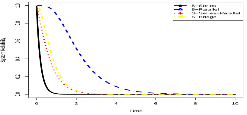
four examples of coherent systems, with Ri(t) = exp(−λt), i= 1, . . . , K, the system reliability functions are

Rser(t;λ, K) = exp(−Kλt);

Rpar(t;λ, K) = 1−[1−exp(−λt)]K;

Rserpar(t;λ) = exp(−λt)[1−(1−exp(−λt))2];

Rbr(t;λ) = 2 exp{−2λt}+ 2 exp{−3λt}+ 2 exp{−5λt} −5 exp{−4λt}.

When λ = 1 and K = 5, these system reliability functions are plotted in Figure 4.1.

An important concept in reliability is measuring the relative importance of each of

(36)

0 2 4 6 8 10

0.0

0.2

0.4

0.6

0.8

1.0

Time

System Reliability

● 5−Series 5−Parallel

3−Series−Parallel 5−Bridge

Figure 4.1 System reliability functions for the series, parallel, series-parallel, and bridge systems when the components have common unit exponential lifetimes and there are 5 components in the series and parallel systems.

importance (cf., (3)). We focus on the so-called reliability importance measure as

this will play an important role in the improved estimation of the system reliability.

The reliability importance of component j in aK-component system with reliability

function hφ(·) is

Iφ(j;p) =

∂hφ(p1,· · · , pj−1, pj, pj+1,· · · , pK)

∂pj

=hφ(p,1j)−hφ(p,0j). (4.14)

This measures how much system reliability changes when the reliability of component

j changes, with the reliabilities of the other components remaining the same. For a

coherent system, the reliability importance of a component is positive. As examples,

the reliability importance of the jth component in a series system is

Iser(j;p) =

hser(p)

pj

, j = 1, . . . , K,

showing that in a series system the weakest (least reliable) component is the most

(37)

reliability importance of thejth component is

Ipar(j;p) =

1−hpar(p) 1−pj

, j = 1, . . . , K,

indicating that the most reliable component is the most important component in a

parallel system. For the 3-component series-parallel system, the reliability importance

of the three components are

Iserpar(1;p) = 1−(1−p2)(1−p3);

Iserpar(2;p) =p1(1−p3);

Iserpar(3;p) =p1(1−p2).

Evaluated at p = (p, p, p), they become Iserpar(1;p) = p(2−p) and Iserpar(2;p) =

Iserpar(3;p) =p(1−p), which confirms the intuitive result that when the components are equally reliable, the component in series (component 1) is the most important

component. In general, however, component 1 is not always the most important.

For instance, if components 2 and 3 are equally reliable with reliability p2, then the

reliability importance of components 1, 2 and 3 become

Iserpar(1; (p1, p2, p2)) =p2(2−p2);

Iserpar(2; (p1, p2, p2)) =Iserpar(3; (p1, p2, p2)) = p1(1−p2).

In this case, component 2 (and 3) is more important than component 1 whenever

p1(1−p2)> p2(2−p2),

or equivalently,

p1 >

p2(2−p2) 1−p2

(38)

4.2 Statistical Model and Data Structure

We now consider the problem of estimating the system reliability function on the basis

of observed data from the system or its components. We suppose that the system has

K components and the observed data will be theK components time-to-failures, but

which could be right-censored by the system lifetime or the end of monitoring period.

We letTj denote the time-to-failure of componentj, and we assume that theTj’s are

independent of each other. We denote byRj(·;θj) the reliability function ofTj, where

θj ∈Θj with the parameter space Θj an open subset of <mj. Furthermore, note that

it is possible that there could be common parameters among the (θj, j = 1,2, . . . , K).

We also assume that the system structure function φ(·) is known, hence we also know the reliability function hφ(p). The system reliability function RS(·) can there-fore be expressed via

RS(t) = RS(t;θ1,θ2, . . . ,θK)

= hφ[R1(t;θ1), R2(t;θ2), . . . , RK(t;θK)]. (4.15)

Suppose there arenidentical systems, so that the observable component lifetimes are

{Tij :i= 1,2, . . . , n;j = 1,2, . . . , K}.

We assume that the Tij’s are independent, and that for each j, (Tij, i = 1,2, . . . , n)

are identically-distributed with reliability functionRj(·;θj). However, in practice, the exact values of the Tij’s are not all observable. Rather, they could be right-censored

by either the system life or by the monitoring period. The observable right-censored

data is

D ={(Zij, δij) :i= 1,2, . . . , n;j = 1,2, . . . , K} (4.16) where δij = 1 means that Tij =Zij, whereas δij = 0 means that Tij > Zij. We shall

(39)

bound of monitoring time for the ith system) and also the system life Si, and

Zij = min{Tij,min(Ci, Si)} and δij =I{Tij ≤min(Ci, Si)}.

On the basis of this observable dataD, it is of interest to estimate the system

reliabil-ity function given in (4.15). A simple estimator of the system reliabilreliabil-ity function is to

utilize only the observed system lifetimes, the Si’s. However, these system lives may

be right-censored by theCi’s, so that we may only be able to observeZi = min(Si, Ci)

and δi = I{Si ≤ Ci} for i = 1,2, . . . , n. If the component lifetime distributions are governed by just one parameter vector, then a parametric approach to estimating this

parameter may be possible, for example when all the component lifetime distributions

are all exponential with rate parameter λ. When component level data is available,

we could improve the estimation of system reliability by utilizing the information on

the internal structure. The lifetime of components are independent with reliability

function

Rj(t;θj) = 1−Fj(t;θj), j = 1· · ·K.

Classically, the estimator of the system reliability function,RS(t), is given by

ˆ

RS(t) = hφ[ ˆR1(t),· · · ,RˆK(t)],

where ˆRj(·) is the MLE of component reliability based on (Zj,δj) ={(Zij, δij) : i= 1,2, . . . , n}. In the parametric setting, ˆRj(t) =Rj(t,θˆj), where θˆj is the MLE ofθj. For component j, to find θˆj, denote the density associated with component j

by fj(t;θj), so the likelihood function based on the completely observed lifetimes of

component j is given by

L(θj,|t1j, . . . , tnj) = n Y

i=1

fj(tij|θj).

In the presence of right-censoring, the likelihood function based on the observed

censored data for component j becomes

Lj(θj; (Zj,δj)) = n Y

(40)

This likelihood could be maximized with respect to θj to obtain the ML estimate

ˆ

θj, which will be a function of the (zij, δij), i = 1,2, . . . , n. The resulting system

reliability function estimator is

˜

RS(t) =hφ[R1(t; ˆθ1), R2(t; ˆθ2), . . . , RK(t; ˆθK)]. (4.17)

From the theory of ML estimators for right-censored data (cf., (2)) under

para-metric models, as n → ∞, we have that

(ˆθ1, . . . ,θˆK)∼AN

(θ1, . . . ,θK), 1

nBD

h

I−1₁ , . . . ,I−1_K i

(4.18)

where I−1_j is the inverse of the Fisher information matrix for the jth component,

and BD means ‘block diagonal’. Assuming no common parameters among the K

components, by using the Delta-Method, we find that, asn → ∞, ˜

RS(t)∼AN 

R_S(t),

1

n

K X

j=1

Iφ(j;t) •

R

T

j (t)I −1 j

•

Rj (t)Iφ(j;t) 



with

•

Rj (t) =

∂ ∂θj

R(t;θj).

In principle, this asymptotic variance could be estimated, though the difficulty may

depend on the structure function and/or distributional form of the Rj’s. Later we

will instead perform comparisons through numerical simulations.

4.3 Improved Estimation Through Shrinkage Idea

Suppose that the component level data are available. The estimation of the

param-eters, (θj, j = 1,2, . . . , K), becomes a problem of simultaneous estimation. In this

context, the problem is to estimate simultaneously the reliability of all components

in the system. Thus, we propose an improved estimator following the idea of James

and Stein(13). Consider estimators of component reliabilities of the form

˜

(41)

where ˆRj(t) = Ri(t,θˆj) is the ML estimator of Rj(t) based on (Zj,δj) under the

assumed parametric model. The system reliability estimator then becomes

ˆ

RS(t;c) = hφ[ ˜R1(t;c),· · · ,R˜K(t;c)]

= hφ{[R1(t;θˆ1)]c,· · · ,[RK(t;θˆK)]c}.

Notice that when c = 1, we obtain the standard ML estimator discussed in the

preceding subsection. If ˆΛj(t) denotes the estimator of the cumulative hazard function

for componentj, according to the relationship mentioned in (4.1), we have

[ ˆRj(t)]c = exp[−cΛˆj(t)].

Thus, we are essentially putting a shrinkage coefficient on the ML estimators of the

cumulative hazard functions. We remark at this point that it is not always the case

that the optimalc∗ is less than 1, so that in some cases, instead of shrinking, we are

expanding the estimators!

The goal is to find the optimal c in terms of a global risk function for the system

reliability estimator. If the optimal shrinkage coefficient isc∗, the improved estimator

of system reliability becomes

ˆ

RS(t;c∗) =hφ{[R1(t,θˆ1)]c

∗

,· · · ,[ ˆRK(t,θˆK)]c

∗

}.

However, the optimal c∗ may depend on the unknown parameters (θ1,· · ·,θK). Therefore, we also need to find an estimator of c∗, denoted by ˆc∗. An intuitive

and simple way to obtain an estimator ofc∗ is to simply replace the unknown θj’s in

the c∗ expression with their corresponding MLEs. The final estimator becomes

ˇ

RS(t) = hφ{[R1(t,θˆ1)]ˆc

∗

,· · · ,[ ˆRK(t,θˆK)]ˆc

∗

(42)

4.4 Evaluating the Estimators

From a decision-theoretic viewpoint, the performance of an estimator a(·) of R(·) =

RS(·) will be evaluated under the following class of loss functions,

L(R, a) =−

Z

|R(t)−a(t)|k_h₍_R₍_t₎₎_dR₍_t₎_. _(4.20)

whereh(·) is a positive function. Note that the negative sign is because the differen-tial element dR(t) is negative since R(·) is a non-increasing functions. The notation

−dR(t) = dF(t) will be used interchangeably, where F is the associated distribu-tion funcdistribu-tion. The decision problem of estimating RS, when using this class of loss

function, becomes invariant with respect to the group of monotone increasing

trans-formations on the lifetimes. A special member of this class of loss functions is the

weighted Cramer-von Mises loss function given by

L(R, a) = −

Z [R(t)−a(t)]2

R(t)(1−R(t))dR(t).

This loss function is a global loss function and can be viewed as the weighted squared

losses aggregated (integrated) over time.

The expected loss or risk function is then given by

Risk(R, a) = EL(R, a) = E

"

−

Z [R(t)−a(t)]2

R(t)(1−R(t))dR(t)

#

, (4.21)

with the expectation taken with respect to the random elements in the estimator

a(t). To find the optimal coefficient c, ˆRS(t;c) is plugged into the risk function and

then the risk is minimized with respect toc. To simplify notation,Risk(c) is used to

(43)

To demonstrate the existence of an optimal c, notice that as c→ ∞,

Risk(c) = E

"

Z [h

φ{[R1(t;θˆ1)]c,· · ·,[RK(t;θˆK)]c} −R(t)]2

R(t)(1−R(t)) dF(t)

#

→ E

"

Z [0−R(t)]2

R(t)(1−R(t))dF(t)

#

=

Z _R(_t)

1−R(t)dF(t) = ∞.

Similarly, when c→0,

Risk(c)→

Z 1−R(t)

R(t) dF(t) =∞.

Therefore, since for every finitec > 0,Risk(c) is finite, and since Risk(c) is a

contin-uous function of c, there exists a value of c, denoted by c∗ ∈ [0,∞), that minimizes the risk function Risk(c).

Using properties of maximum likelihood estimators, as n → ∞, θˆj converges in probability to θj, j = 1,· · · , K. Thus, when n → ∞, the optimal c∗ that minimizes the expected loss converges in probability to c∗ = 1. Therefore, for large n, the