Unaligned Rebound Attack:
Application to Keccak
Alexandre Duc1,∗, Jian Guo2,†, Thomas Peyrin3,‡, and Lei Wei3,§ 1
Ecole Polytechnique F´ed´erale de Lausanne, Switzerland
2
Institute for Infocomm Research, Singapore
3
Nanyang Technological University, Singapore
{ntu.guo,thomas.peyrin}@gmail.com [email protected]
Abstract. We analyze the internal permutations of Keccak, one of the NIST SHA-3 competition
finalists, in regard to differential properties. By carefully studying the elements composing those per-mutations, we are able to derive most of the best known differential paths for up to 5 rounds. We use these differential paths in a rebound attack setting and adapt this powerful freedom degrees utiliza-tion in order to derive distinguishers for up to 8 rounds of the internal permutautiliza-tions of the submitted version ofKeccak. The complexity of the 8 round distinguisher is 2491.47. Our results have been
im-plemented and verified experimentally on a small version ofKeccak. This is currently the best known
differential attack against the internal permutations ofKeccak.
Key words:Keccak, SHA-3, hash function, differential cryptanalysis, rebound attack.
1
Introduction
Cryptographic hash functions are used in many applications such as digital signatures, authentication schemes or message integrity and they are among the most important tools in cryptography. Informally, a hash function H is a function that takes an arbitrarily long message as input and outputs a fixed-length hash value of sizenbits. Even if hash functions are traditionally used to simulate the behavior of a random oracle [3], classical security requirements are collision resistance and (second)-preimage resistance. Namely, it should be impossible for an adversary to find a collision (two distinct messages that lead to the same hash value) in less than 2n/2 hash computations, or a (second)-preimage (a message hashing to a given
challenge) in less than 2n hash computations. Of course, in the ideal case an attacker should also not be able to distinguish the hash function from a random oracle.
Recently, most of the standardized hash functions [25, 20] have suffered from serious collision attacks [29, 28]. As a response the NIST launched in 2007 theSHA-3competition [21] that will lead to the future hash function standard. 5 candidates made it to the final round, and Keccak [9] is among them. Compared
to its opponents, this hash function presents the particularity to be a sponge function [5]. The submitted versions ofKeccak to the SHA-3 competition use as main component an internal permutation P of 1600
bits. In the original submission [6] the internal permutation used 18 rounds and the tweaked versions [7] went up to 24 rounds.
∗Part of the work was done while the author was visiting Nanyang Technological University, supported by the
NTU NAP Startup Grant M58110000. The work described in this paper has also partially been supported by the European Commission through the ICT Program under contract ICT-2007-216646 ECRYPT II.
†Part of the work was done while the author was visiting Tsinghua University, supported by the National Natural
Science Foundation of China under grant No. 61133013 and No. 60931160442.
‡The author is supported by the Lee Kuan Yew Postdoctoral Fellowship 2011 and the Singapore National Research
Foundation Fellowship 2012.
§The author is supported by the Singapore National Research Foundation under Research Grant
Like any construction that builds a hash function from a subcomponent, the cryptographic quality of this internal permutation is very important for a sponge construction. Therefore, this permutationP should not present any structural flaw, or should not be distinguishable from a randomly chosen permutation. Previous cryptanalysis have not endangered the Keccak security so far. Zero-sum distinguishers [2] can
reach an important number of rounds, but generally with a very high complexity. For example, the latest results [11] provide zero-sum partitions distinguishers for the full 24-round 1600-bit internal permutation with a complexity of 21575. When looking at smaller number of rounds the complexity would decrease, but it
is unclear how one can describe the partition of a 1600-bit internal state without using theKeccakround
inside the definition of the partition. Moreover, such zero-sum properties seem very hard to exploit when the attacker aims at the whole hash function. On the other side, more classical preimage attack on 3 rounds using SAT-solvers have been demonstrated [19]. Finally, Bernstein published [4] a 2511.5 computations
(second)-preimage attack on 8 rounds that allows a workload reduction of only half a bit over the generic complexity with an important memory cost of 2508.
Our contributions. In this article, we analyze the differential cryptanalysis resistance of the Keccak
internal permutation. More precisely, we first introduce a new and generic method that looks for good differ-ential paths for all theKeccakinternal permutations, and we obtain the currently best known differential
paths. We then describe a simple method to utilize the available freedom degrees which allows us to derive distinguishers for reduced variants of theKeccak internal permutations with low complexity. Finally, we
apply the idea of rebound attack [18] toKeccak. This application is far from being trivial and requires a
careful analysis of many technical details in order to model the behavior of the attack. This technique is in particular much more complicated to apply to Keccak than to AESor to other 4-bit Sbox hash
func-tions [24, 14]. One reason for that is thatKeccak hasweak alignment [8]. This is why we call our attack
“unaligned rebound attack”. The model introduced has been verified experimentally on a small version of
Keccakand we eventually obtained differential distinguishers for up to 8 rounds of the submitted version
ofKeccakto the SHA-3competition. In order to demonstrate why differential analysis is in general more
relevant than zero-sum ones in regards to the full hash function, we applied our techniques to the recent
Keccak challenges [27] and managed to obtain the currently best known collision attack for up to two
rounds.
Outline. In Section 2, we first briefly describe the Keccak family of hash functions. We describe our
differential path search algorithm in Section 3 and we derive simple differential distinguishers from it in Section 4. We present our theoretical model and we apply the rebound attack on Keccak in Section 5.
We show how to reduce the complexity of the attack in Section 6. Finally, we present our results and draw conclusions in Section 7.
2
The
Keccak
Hash Function Family
Keccak[9, 10] is a family of variable length output hash functions based on the sponge construction [5]. In Keccakfamily, the underlying function is a permutation chosen from a set of sevenKeccak-f
permuta-tions, denoted asKeccak-f[b] where b∈ {1600,800,400,200,100,50,25}is the permutation width as well
as the internal state size of the hash function. TheKeccak family is parametrized by anr-bit bitrate and
c-bit capacity with b=r+c.
A fixed lengthn-bit hash value for aKeccakhash function is obtained by truncating the output of the
hash function to the first n bits and this function is denoted byKeccakn. For these variants, if at least
2n (second) preimage resistance security is desired then the parameterc is chosen such thatc ≥2n. The proposed version ofKeccakfor the SHA-3 standardization usesKeccak-f[1600] as internal permutation.
The default variant ofKeccak family is denoted by Keccak-[] and it has parameters r= 1024,c= 576
for any output lengthn.
2.1 The domain extension algorithm
Sponge is an iterated construction to build a functionF :{0,1}∗ → {0,1}∗ by using a fixed length
initial value of the state is zero and the input message is padded such that it is a multiple ofr-bit message blocks (and the last message block is different than zero).
Message processing using sponge construction has two stages: absorbing phase and squeezing phase. In the absorbing phase, r-bit message blocks are xor-ed with the first r bits of the b-bit state, interleaved with the applications off until all blocks are processed. In the squeezing phase, depending on the required number of output bits n, the firstr bits of the state are returned as output blocks, interleaved with the applications off untilnbits are returned.
2.2 The Keccak-f permutations
The internal state of theKeccakfamily can be viewed as a bit array of 5×5 lanes, each of lengthw= 2ℓ
whereℓ∈ {0,1,2,3,4,5,6}andb= 25w. The state can also be described as a three dimensional array of bits defined bya[5][5][w]. A bit position (x, y, z) in the state is given bya[x][y][z] wherexandycoordinates are taken over modulo 5 and thez coordinate is taken over modulow. Alaneof the internal state atcolumn x
androw y is represented bya[x][y][·], while aslice of the internal state atwidth zis represented bya[·][·][z].
Keccak-f[b] is an iterated permutation consisting of a sequence ofnr rounds indexed from 0 tonr−1
and the number of rounds are given by nr= 12 + 2ℓ. A roundR consists of a transformation of five step mappings and is defined by:
R=ι◦χ◦π◦ρ◦θ
These step mappings are discussed below where the operation + indicates bitwise addition.
θ mapping. This linear mapping intends to provide diffusion for the state and is defined for every x, y
andz by:
θ:a[x][y][z]←a[x][y][z] +
4
M
y′=0
a[x−1][y′][z] +
4
M
y′=0
a[x+ 1][y′][z−1]
That is, the bitwise sum of the two columnsa[x−1][·][z] anda[x+ 1][·][z−1] is added to each bita[x][y][z] of the state.
ρ mapping. This linear mapping intends to provide diffusion between the slices of the state through intra-lane bit translations. For everyx,y andz:
ρ:a[x][y][z]←a[x][y][z+T(x, y)]
whereT(x, y) is a translation constant. That is, all bit positions in each lane are translated by a constant amount that depends on the columnxand rowy considered.
π mapping. This linear mapping intends to provide diffusion in the state through transposition of the lanes. More precisely, it is defined for everyx, yand zas:
π:a[x′][y′][z]←a[x][y][z], with
x′ y′
=
0 1 2 3
·
x y
Since this results in transposition of bits into a same slice, this mapping is an intra-slice transposition.
χmapping. This is the only non-linear mapping ofKeccak-f and is defined for everyx,y andzby:
χ:a[x][y][z]←a[x][y][z] + ((¬a[x+ 1][y][z])∧a[x+ 2][y][z])
This mapping is similar to an Sbox applied independently to each 5-bit row of the state and can be computed in parallel to all rows. We represent bys= 5wthe number of Sboxes/rows inKeccakinternal state. Here
ι mapping. For every round Rof theKeccak-f permutation, this mapping adds constants derived from
an LFSR (see [9] for details) to the lanea[0][0][·]. These constants are different in every roundi:
ι:a[0][0][·]←a[0][0][·] + RC[i]
This mapping aims at destroying the symmetry introduced by the identical nature of the remaining mappings in every round of theKeccak-f permutation.
We refer to the Keccakspecifications document [9] for all the translation and round constants.
3
Finding Differential Paths for
Keccak
-f
Internal Permutations
Before describing how we use the freedom degrees in a rebound attack setting, we first study how to find “good” differential paths for all Keccakvariants. In this section, we describe our differential finding
algorithms. We start by recalling several special properties of the mappingsθandχin the round function, followed by our algorithm which provides most of the best known differential paths for theKeccakinternal
permutations. In particular, we provide the currently best known 3, 4 and 5-round differential paths for
Keccak-f[1600], the internal permutation from the submitted version ofKeccak.
3.1 Special properties ofθ and χ
Theθ mapping updates each state bita[x][y][z] by adding the bitwise sum of the two columnsa[x−1][.][z] and a[x+ 1][.][z−1]. When every column sums to 0, θ acts as identity. This is noted by the Keccak
designers [9, Section 2.4.3], and the set of the states with all columns sums to 0 is called column parity kernel, orCP-kernel for short. Since θis linear, this property applies not only to the state values, but also to differentials. Whileθ expands a single bit difference into at most 11 bits (2 columns and the bit itself), it has no influence,i.e., acts as identity, on differences in the CP-kernel. This property will be intensively used in finding low Hamming weight bitwise differentials. Another interesting property is thatθ−1diffuses
much faster thanθ, i.e., a single bit difference can be propagated to about half state bits throughθ−1 [9,
Section 2.3.2]. However, the output ofθ−1 is extremely regular when the Hamming weight of the input is
low.
Theχlayer updates each bita[x, y, z] by adding ((¬a[x+1, y, z])∧a[x+2, y, z]). It is a row-wise operation and thus can also be viewed as a 5-bit Sbox. Similar to the analysis of other Sboxes, we build the differential distribution table (DDT), as shown in Table 3 in Appendix B. We remark that when a single difference is present,χacts as identity with the best probability 2−2, while input differences with more active bits tends
to lead to more possible output differences, but with lower probability. It is also interesting to note that given an input difference toχ, all possible output differences occur with same probability. However this is not the case forχ−1 (the DDT forχ−1can be derived from Table 3).
3.2 First tools
Our goal is to derive “good” bitwise differential paths by maintaining the bit difference Hamming weight as low as possible. Theι permutation adds predefined constants to the first lane, and hence has no essential influences when such differentials are considered. For the rest of the paper, we will ignore this layer. We note thatθ,ρandπare all linear mappings, whileχacts as a non-linear Sbox. Furthermore,ρandπdo not change the number of active bits in a differential path, but only bit positions. Hence,θ and χ are critical when looking for a “good” differential path. Since χ is followed by θ in the next round (ignoring ι), we consider these two mappings together by treating a slice of the state as a unit, and try to find the potential best mapping of the slice throughχwith the following two rules.
1. Given an input difference of the slice, i.e., 5 row differences, find all possible output differences by looking into the DDT table. Then among all combinations of solutions of the 5 rows, choose the output combinations with minimum number of columns with odd parity.
Rule 1 aims at reducing the amount of active bits after applyingθ by choosing each slice of the output of theχ closest to the CP-kernel (i.e.,with even parity for most columns), and rule 2 further reduces the amount of active bits within the columns. Although this strategy may not lead to the minimum number of active bits after θ in the entire state (the full Keccak-f[1600] state is too large to precompute the best
mappings for the whole state), it finds the best slice-wise mappings with help of a table of size 225 (tricks
like removing the ordering of the rows reduce the table size to about 218). We call this tableχ-slice-table.
3.3 Algorithm for differential path search
Denoteλ=π◦ρ◦θ(all linear mappings), and the state at round ibefore (resp. after) applying the linear layerλasai (resp.bi). We start our search froma1,i.e.,the input state to the second round, and compute
backwards for one round, and few rounds forwards, as shown below.
a0
λ−1 ←−−b0
χ−1
←−−a1−→λ b1
χ −→a2
λ −→b2
χ −→a3
λ −→b3· · ·
The forward part is longer than the backward part because the diffusion of θ−1 is much better than for θ, thus, it will be easier for us to control the bit differences Hamming weight for several forward rounds (instead of backward rounds).
We choosea1from the CP-Kernel. However, it is impossible to enumerate all ( 50+ 25+ 54)320= 21280
combinations. We further restrict to a subset of the CP-Kernel with at most 8 active bits and each column having exactly 0 or 2 active bits. Note also that any bitwise differential path is invariant through position rotation along the z axis, so we have to run through a set of size about 236. A brute-force search on this
set using our two rules stated previously finds 3-round differential paths with probability 2−32, 4-round
differential paths with probability 2−142 and 5-round paths with probability 2−709 for Keccak-f[1600],
with examples shown in Table 6, 7 and 8 in Appendix D, respectively. We provide also in Table 1 all the best differential path probabilities found for allKeccakinternal permutation sizes.
Table 1.Best differential path results for each version ofKeccakinternal permutations, for 1 up to 5 rounds. The
detailed differential paths forKeccak-f[1600] are shown in Appendix D. Paths in bold are new results we found
with the method presented in this paper.
b best differential path probability (successive differential complexity of the rounds)
1 rd 2 rds 3 rds 4 rds 5 rds
100 2−2
(2) 2−8
(4 - 4) 2−19
(4 - 8 - 7) 2−30
(4 - 8 - 10 - 8) 2−54
(4 - 8 - 10 - 8 - 24) 200 2−2
(2) 2−8
(4 - 4) 2−20
(4 - 8 - 8) 2−46
(11 - 9 - 8 - 8) 2−108
(8 - 16 - 20 - 16 - 48) 400 2−2
(2) 2−8
(4 - 4) 2−24
(8 - 8 - 8) 2−84
(16 - 14 - 12 - 42) 2−216
(16 - 32 - 40 - 32 - 96) 800 2−2
(2) 2−8
(4 - 4) 2−32
(4 - 4 - 24) 2−109
(12 - 12 - 12 - 73) 2−432
(32 - 64 - 80 - 64 - 192) 1600 2−2
(2) 2−8
(4 - 4) 2−32(4 - 4 - 24) 2−142(12 - 12 - 12 - 106) 2−709(16 - 16 - 16 - 114 - 547) A better path (2−510
) was found in-dependently [23]
Comment. In the reference document [9], among other methods, theKeccakdesigners looked for special
differential paths to motivate their choice of the step mappings. In their model, the input states to theχof the first two rounds are forced to fall entirely inside the CP-kernel. The best 3-round path they could find forKeccak-f[1600] has probability 2−35. Note also that no 4-round and 5-round path is obtained. Their
results were up to now the best published differential paths forKeccak. As shown in Table 1, our model
outperforms in most cases theKeccakdesigners model by removing this strong restriction onχand using
4
Simple Distinguishers for the Reduced
Keccak
Internal Permutations
Once the differential paths obtained, we can concentrate our efforts on how to use at best the freedom degrees available in order to reduce the complexity required to find a valid pair for the differential trails or to increase the amount of rounds attacked. We present in this section a very simple method that allows to obtain low complexity distinguishers on a few rounds of theKeccak internal permutations.
4.1 A very simple freedom degrees fixing method
We first describe an extremely simple way of using the available freedom degrees, which are exactly theb-bit value of the internal state (since we already fixed the differential path). For all the best differential paths found from Table 1, we can extend them by one round to the left or to the right by simply picking some valid Sboxes differential transitions. Obviously, this is going to add a lot of new constraints because the number of active Sboxes will explode in this newly added round and it will force the differential probability to be very low overall. However, we can use our available freedom degrees specifically for this round so that its cost is null. One simply handles each of the active Sboxes differential transitions for this round one by one, independently, by fixing a valid value for the active Sboxes. In terms of freedom degrees consumption for this extra round, in the worst case we have alls Sboxes active and a differential transition probability of 2−4for each of them. Thus, we are ensured to have at least 25s−4s= 2sfreedom degrees remaining after handling this extra round.
Let us assume for example that we start from the 4-round differential path for Keccak-f[1600], with
differential probability 2−142. One can obtain a 5 round path by adding one round to the left but the number
of conditions for this new round will be huge. Therefore, we simply identify all the active Sboxes for this fifth round and we fix the value for them so that the expected differential transitions are verified. Overall, the attacker finds a valid pair of internal state values for the 5-round differential path only with complexity 2142 (we are ensured to have at least 2320freedom degrees to handle the 2−142probability). Note that some
more involved freedom degree methods (such as message modification [28]) might even allow to also control some of the conditions of the original differential path, thus further reducing the complexity.
4.2 The generic case
At the present time, we are able to find valid pairs of internal state values for some differential paths on a few rounds with a rather low complexity. Said in other words, we are able to compute internal state value pairs with a predetermined input/output difference. A direct application from this is to derive distinguishers. For a randomly chosen permutation ofbbits, finding a pair of inputs with a predetermined difference that maps to a predetermined output difference costs 2b computations. Indeed, since the input and the output differences are fixed, the attacker can not apply any birthday-paradox technique. Those distinguishers are called “limited-birthday distinguishers” and can be generalized in the following way (we refer to [12] for more details): for a randomly chosen b-bit permutation, the problem of mapping an input difference from a subset of sizeI to an output difference from a subset of size J requires max{p
2b/J,2b/(I·J)} calls to permutation (while assuming without loss of generality since we are dealing with a permutation thatI≤J). Using the freedom degrees technique from the previous section and reading Table 1, we are for example able to obtain a distinguisher for 5 rounds of theKeccak-f[1600] internal permutation with complexity
2142 (while the generic case is 21600).
4.3 Extending the differential path
Since for many of our distinguishers, the gap between our attack and the generic case complexity is very big, we can try to reach a few more rounds without increasing the complexity. Indeed, by analyzing how the differences will propagate forward from the output and backward from the input of our differential path, we will be able to determine the size of the possible input differences set and the possible output differences set.
and we obtain the difference mask at the input ofχ. Now, for each active Sbox, knowing exactly its input difference, we can check with the DDT fromχ (Table 3 in the Appendix B) that only a subset of the 25
possibles output differences can be reached. Therefore, the sizeΓout
of the set of reachable output differences after applying this extra round is bounded and this bound can be computed exactly using the DDT from
χ.
For the backward case (i.e. when adding a round to the left), we start from the fully determined difference on the input of the differential path. Then, reading at the DDT from χ−1, one can check that one active
Sbox can produce at most a certain small subset of the 25 possible input differences. Therefore, the size Γin of the set of reachable input differences after inverting this χlayer is bounded and this bound can be
computed exactly using the DDT fromχ−1. Note that continuing to invert the extra round by computing θ−1,ρ−1andπ−1will not modify the size of this set.
To conclude, using a r-round path from Table 1 with differential probability p, we extend it by one more round in order to find valid internal state pairs for this new (r+ 1)-round differential path with p−1
computations (see Section 4.1). Then, using the limited-birthday distinguishers, one can derive a (r+ 3)-round distinguisher for theKeccakinternal permutation with complexityp−1, if
p−1<max{q2b/J,2b/(I·J)}
whereI=Γout
andJ =Γin
ifΓout≤
Γin
; I=Γin
andJ =Γout
otherwise.
Continuing our example with the 4-round differential path forKeccak-f[1600] from Table 1, we have
Γin
= 21064 and Γout
= 2576 for a 7-round distinguisher of the internal permutation. Thus the generic
complexity to find such constraint pairs is 2268 computations which is much higher than 2142. All the
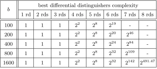
distinguishers we obtain with this method are summarized in Table 2.
Note that the reader might be concerned by the fact that the sizesΓinandΓoutof the reachable differences
sets can be very big and might be not easy to describe in a compact way in our distinguisher. However, we emphasize that all the reachable differences on the output (resp. input) are actually built from the independent combinations of all the possible output differences (resp. input differences) of all active Sboxes in the last round (resp. first round). Therefore, the description of this set is easily done by identifying the reachable output differences (resp. input differences) for all the Sboxes independently.
5
The Rebound Attack on
Keccak
The rebound attack is a freedom degrees utilization technique that was first proposed by Mendel et al.
in [18] as an analysis of round-reduced Grøstl andWhirlpool. It was then improved in [17, 16, 12, 26] to analyzeAESandAES-like permutations and also ARX ciphers [15].
With the help of rebound techniques, we show in this section how to extend the number of attacked rounds significantly, but for a higher complexity. We will see that the application of the rebound attack for Keccak seems quite difficult. Indeed, the situation for Keccak is not as pleasant as the AES-like
permutations case where the utilization of truncated differential paths (i.e. path for which one only checks if one cell is active or inactive, without caring about the actual difference value) makes the application of rebound attacks very easy to handle.
5.1 The original rebound attack
LetP denote a permutation, which can be divided into 3 sub-permutations,i.e., P =EF ◦EI◦EB. The rebound attack works in two phases.
• Inbound phase or controlled rounds: this phase usually starts with several chosen input/output differences ofEI that are propagated through linear layers forward and backward. Then, one can carry out meet-in-the-middle (MITM) match for differences through a single Sbox layer in EI and generate all possible value pairs validating the matches.
In most cases, the inbound phase can be done fast due to the MITM nature and generates solution pairs with very low average complexity. Hence, attackers usually choose the position of EI in the differential path so that it covers a low probability portion of the trail in order to increase the success probability of the outbound phase. For example when dealing with the 128-bitAES internal permutation, this MITM is performed on sixteen parallel 8-bit Sboxes. If the match is done with k Sboxes being active and since a random 8-bit input/output difference can be matched with probability 1/2 through a singleAESSbox, one needs to try at least 2k input/output difference pairs ofE
I in order to hope having one matching candidate for the inbound phase. However, once a match is found one can generate about 2k solution values from it, thus leading to an average cost of about one operation per solution for the controlled rounds. The final goal of the attacker is then to generate enough inbound phase solution values such that one of them also verifies the forward and backward outbound trails, i.e at leastp−B1·pF−1 pairs need to be tested ifpB and pF are the respective backward and forward differential probability (DP) of the outbound trail.
The SuperSbox technique [16, 12] extends theEI from one Sbox layer to two Sbox layers for anAES-like permutation, by considering two consecutiveAES-like rounds as one with column-wise SuperSboxes. This technique is possible due to the fact that one can swap few linear operations with the Sbox inAES, so that the two layers of Sboxes in two rounds become close enough to form one SuperSbox layer. However, in the case of Keccak, it seems very hard to form any partition into independent SuperSboxes. For the same
reason, using truncated differential paths seems very difficult for Keccak, as it has recently been shown
in [8].
During the application of rebound attacks, one has to start with several input/output differences of
EI to complete the inbound phase. ForAES-like permutations one can start with truncated differences and thus it is much more handy because this view simplifies a lot the analysis. Indeed, a truncated differential forAES-like permutations can be seen as a collection of several bit differentials, all with the same success probability and the same properties in regards to rebound attacks. Thus, whatever the difference masks considered for the input/output of the controlled rounds, the probabilitiespB andpF will remain the same, so will the probability to get a match inEI or the number of solutions that can be generated from a match. This will not be the case forKeccak as we can not use truncated differential paths and the analysis will
be much more involved.
5.2 Applying the rebound attack for Keccak internal permutations
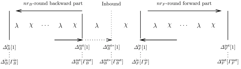
Assume that we know a set of nB differential trails (called backward trails) on nrB Keccak rounds and whose DP is higher or equal topB. For the moment, we want all these backward paths to share the same input difference mask∆in
B and we denote by∆
out
B [i] the output difference mask of thei-th trail of the set. Similarly, we consider that we also know a set ofnF differential trails (calledforward trails) onnrF Keccak rounds and whose DP is higher or equal topF. We want all those forward paths to share the same output difference mask∆out
F and we denote by∆
in
F[i] the input difference mask of thei-th trail of the set.
λ
χ
. . .
λ
χ
λ
χ
λ
χ
. . .
λ
χ
∆inB[1] ∆
out
B [1] ∆ out∗
B [1] ∆ in
F[1] ∆
out F [1]
..
. ... ... ... ...
∆in B[Γ
in
B] ∆
out B [Γ
out B ] ∆
out∗
B [Γ out B ] ∆
in F[Γ
in
F] ∆
out F [Γ
out F ]
nrB-round backward part Inbound nrF-round forward part
Fig. 1.Rebound attack onKeccak
match is possible from a given element of the backward set and a given element of the forward set, and we denote byNmatchthe number of solution values that can be generated once a match has been obtained.
For this connection to be possible, we need the inbound phase to be a valid differential path, that is we need to find a valid differential path from a∆out∗
B to a∆
in
F. By using random∆
out∗
B and∆
in
F this will happen in general with very small probability, because we need the very same set of Sboxes to be active/inactive in both forward and backward difference masks to have a chance to get a match. Even if the set of active Sboxes matches, we still require the differential transitions through all the active Sboxes to be possible.
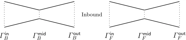
We can generalize a bit this approach by allowing a fixed set of differences ∆in
B (resp.∆
out
F ) instead of just one. We call Γin
B (resp. Γ
out
B ) the size of the set of possible ∆
in
B (resp. ∆
out
B ) values for the backward paths. Similarly, we callΓin
F (resp.Γ
out
F ) the size of the set of possible∆
in
F (resp.∆
out
F ) values for the forward paths. In fact, the number of possible differences in the backward or forward parts will form a butterfly shape (see Figure 2). We callΓmid
B (resp.Γ
mid
F ) the minimum number of differences in the backward (resp. forward) part.
Γ
inB
Γ
mid
B
Γ
out
B
Γ
in
F
Γ
mid
F
Γ
out F
Inbound
Fig. 2.Number of differences for the rebound attack onKeccak.
The total complexity Cto find one valid internal state pair for the (nrB+nrF+ 1)-round path is
C=nF +nB+ 1
pmatch
·
1
pF·pB·Nmatch
+ 1
pB·pF
, (1)
with
Γout
B ·Γ
in
F = 1
pmatch
·
1
pF ·pB·Nmatch
. (2)
The first two terms are the costs to generate the backward and forward paths. The term ⌈ 1
pF·pB·Nmatch⌉ denotes the number of time we will need to perform the inbound and each inbound costs 1/pmatch. The last
term is the cost for actually performing the outbound phase. The condition (2) is needed since we need enough differences to perform the inbound phase.
Roadmap. For a better understanding of the behavior of the Sboxes in the rebound attack, we will introduce some useful lemmas in Section 5.3. We explain how to prepare the forward and backward differential paths in Section 5.4 and describe the inbound and outbound phases in Section 5.5 and 5.6 respectively. We explain how to relate Sections 5.4, 5.5 and 5.6 in Section 5.7, we show also how we can reduce the complexity of the attack and we give a numerical application of our model. Finally we construct distinguishers from the differential paths in Section 5.8.
5.3 An Ordered Buckets and Balls Problem
We model the active/inactive Sboxes match as alimited capacity ordered buckets and balls problem:4
thes= 5wordered buckets (s= 320 for Keccak-f[1600]) limited to capacity 5 will represent thes5-bit
Sboxes and the xB (resp.xF) balls will stand for the Hamming weight of the difference in ∆outB ∗ (resp. in
∆in
F). Given a setB ofsbuckets in which we randomly throwxBballs and a setF ofsbuckets in which we randomly throwxF balls, we call the result apattern-matchwhen the set of empty buckets inB and F
4
after the experiment are the same.5 Before computing the probability of having a pattern-match, we need
the following lemma.
Lemma 1. The number of possible combinations bbucket(n, s) to placen balls into s buckets of capacity 5
such that no bucket is empty is
bbucket(n, s) :=
s X
i=⌈n/5⌉
(−1)s−i
s
i
5i
n
if s≤n≤5s
0 else.
(3)
Proof. First note that the number of combinations verifies the following recurrence relation:
bbucket(n, s) =
5
1
bbucket(n−1, s−1) +
5
2
bbucket(n−2, s−1) +· · ·+
5
5
bbucket(n−5, s−1),
withbbucket(x, s) = 0 whenx≤0 andbbucket(x,1) = x5
when 0< x≤5 and 0 else. Let’s consider the following generating function:
Gs(x) :=X k≥0
bbucket(k, s)xk .
We have
G1(x) =
5 1 x+ 5 2
x2+· · ·+
5
5
x5= (x+ 1)5
−1.
Hence,P
k≥1bbucket(k, s)xk =
X
k≥1
5 1
bbucket(k−1, s−1) +
5 2
bbucket(k−2, s−1) +· · ·+
5 5
bbucket(k−5, s−1)
xk
=X
k≥1
5 1
bbucket(k−1, s−1)xk+
X
k≥2
5 2
bbucket(k−2, s−1)xk+· · ·+
X
k≥5
5 5
bbucket(k−5, s−1)xk
=X
k≥0
5
1
bbucket(k, s−1)xk·x+
X
k≥0
5
2
bbucket(k, s−1)xk·x2+· · ·+
X
k≥0
5
5
bbucket(k, s−1)xk·x5
=Gs−1(x)·
5 1 x+ 5 2
x2+· · ·+
5
5
x5
=Gs−1(x)· (x+ 1)5−1=Gs(x).
The last equality follows frombbucket(0, s) = 0. LetA:= (x+ 1)5−1. We have
Gs(x) =Gs−1(x)A=G1(x)As−1=As=
s
X
i=0
(−1)s−i
s
i
(x+ 1)5i
= s X i=0 5i X j=0
(−1)s−i
s
i
5i
j
xj . (4)
The number of combinationsbbucket(n, s) we are looking for is the coefficient ofxnin the expressionGs(x) =
P
k≥0bbucket(k, s)xk. By summing in (4) the terms contributing toxn we obtain the wanted result. ⊓⊔
Using (3), we can derive the probabilitypbucket that every bucket contains at least one ball whennballs are
thrown intosbuckets with capacity 5:
pbucket(n, s) :=
bbucket(n, s)
5s n
. (5)
5
The expected number of active buckets whennballs are thrown intosbuckets is given by
Ps
i=0bbucket(n, s−i)· si·(s−i)
5s n
. (6)
We can now relate this lemma to the more general pattern-match problem.
Lemma 2. Given a set ofsbucketsB of capacity5in which we throwxB balls and a set ofsbucketsF in
which we throwxF balls, the probability thatB andF have the same pattern of empty buckets is given by
ppattern(s, xB, xF) = 1
5s xB
5s xF
s
X
i=0
bbucket(xB, s−i)bbucket(xF, s−i)
s
i
,
wherebbucket(x, s)is defined as in(3). The average numbernpatternof non-empty buckets if both experiments
results follow the same pattern is given by
npattern(s, xB, xF) =
Ps
i=0bbucket(xB, s−i)bbucket(xF, s−i) si
(s−i)
Ps
i=0bbucket(xB, s−i)bbucket(xF, s−i) si
.
This model tells us that when the number of balls (i.e., active bits) is not too small on both sides, most of the matches happen when (almost) all the Sboxes are active. Figure 8 in Appendix A depicts this behavior.
A More General Problem. We can also look into a more general problem, i.e., we characterize more precisely how the bits are distributed into the Sboxes.
Lemma 3. The probabilitypdist of distributing randomlynactive bits into s5-bit Sboxes such that exactly
Ai Sboxes contain ibits, for i∈[1,5]is
pdist(A1, A2, A3, A4, A5) :=
s! 51A1 5 2
A2 5 3
A3 5 4
A4 5 5
A5
(s−A1−A2−A3−A4−A5)!A1!A2!A3!A4!A5! 5ns
, (7)
withn=A1+ 2A2+ 3A3+ 4A4+ 5A5.
Important Remark. Since most matches happen when all the Sboxes are active, in order to simplify the analysis, we will use from now on only forward and backward paths such thatall Sboxes are active in theχ layer of the inbound phase.
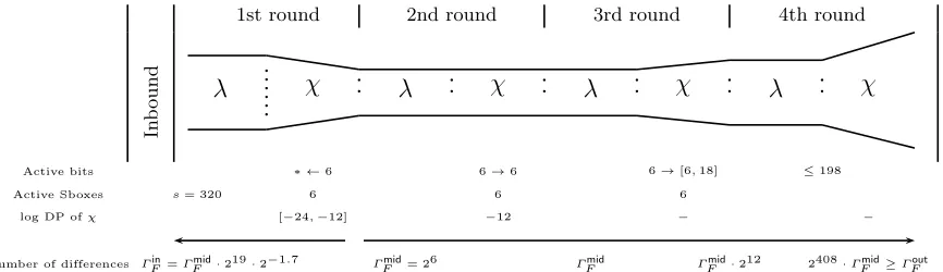
5.4 The differential paths sets
In this section, we explain how we generate the forward and backward paths, since this will have an impact on the derivation ofpmatch andNmatch(this will be handled in the next two sections).
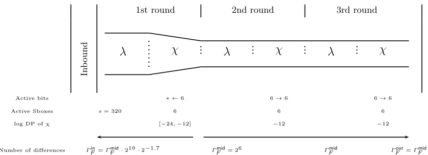
The forward paths. For the forward paths set, we start by choosing a differential trail computed from the previous section and we derive a set from it by exhausting all the possible Sbox differential transitions for the inverse of the χ layer in its first round (all the paths will be the same except the differences on their input and on the input of the χlayer in the first round). For example, we can use the 3 first rounds of the 4-round differential path from Table 7 in Appendix D which have a total success probability 2−36
and present 6 active Sboxes during the χ layer of the first round. Note that we didn’t choose the best 3-round differential path (with success probability 2−32) since it will not provide enough paths (due to its
input difference Hamming weight being too small). We randomize theχ−1 layer differential transitions for the 6 active Sboxes of the first round, and we obtain about 219 distinct trails in total. We analyzed that all the trails of this set have a success probability of at least 2−48 (this is easily obtained with the χ−1
λ
χ
λ
χ
λ
χ
Active bits
Active Sboxes
log DP ofχ
Number of differences
s= 320
ΓFin=ΓFmid·219·2−1.7 ∗ ←6
6
[−24,−12]
ΓFmid= 26
6→6
6
−12
ΓFmid
6→6
6
−12
ΓFout=ΓFmid
1st round 2nd round 3rd round
In b o u n d
Fig. 3.The forward trails. Values are taken from the 3 round differential path from Table 7. The distance between the two lines reflects the number of differences.
distinct input masks (at the first round). Since we previously forced the requirement that all Sboxes must be active for the inbound match, we check experimentally that 217.3 of the 219 members of the set fulfill
this condition.6We callτ
F the ratio of paths that verify this condition over the total number of paths, i.e.,
τF = 2−1.7. Overall, we built a set of 217.3forward differential paths onnrF = 3Keccak-f[1600] rounds, all with DP higher or equal topF = 2−48. We can actually generate 64 times more paths by observing that they are equivalent by translation along theKeccak lane (thez axis). However, these paths will have distinct
output difference masks (the same difference mask rotated along thezaxis), and we haveΓout
F =Γ
mid
F = 26. Thetotal amount of input differences Γin
F is, hence, Γ
in
F :=Γ
mid
F ·217.3 = 223.3 and we have to generate in totalnF =τF·ΓFin= 225 forward differential paths.
λ
χ
λ
χ
λ
χ
Active Sboxes
Hamming weight
log DP ofχ
Number of differences
2X
2X←2X
−4X
ΓBin(X) ΓBin(X)−×ǫ−−→ΓBmid(X) 2X
2X→2X+k
−4X
Γmid B (X)·
2X
k
2k
P5
i=1Ai
n
−2A1−3A2 −4(A3 +A4 +A5 )
Γmid B (X)·
2X
k
2k GB(n)·τfull B
1st round 2nd round 3rd round
In b o u n d
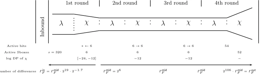
Fig. 4.The backward trails. The distance between the two arrows reflects the number of differences.
The backward paths. Applying the same technique to the backward case does not generate a sufficient amount of output differencesΓout
B , crucial for a rebound-like attack. Thus, concerning the backward paths set, we build another type of 3-round trails. We need first to ensure that we haveenough differential pathsto be able to find a match in the inbound phase, i.e., we wantΓout
B ·Γ
in
F = 1/pmatch· ⌈p 1
F·pB·Nmatch⌉following (2). Moreover, we will require these paths to verify two conditions:
1. First, we need to filter paths that have not all Sboxes active in the χ layer of the inbound phase. Using (5), this happens with a probability about τfull
B :=pbucket(800,320) = 2−15.9 if we assume that
6
The small amount of filtered forward paths (a factor 21.7
about half of the bits are active. This assumption will be verified in our case (and was verified in practice) since our control on the diffusion of the active bits will be reduced greatly.
2. Moreover, all the paths we collect should have a DP of at least pB such that the number of solutions
Nmatchgenerated in the inbound phase is sufficient. Indeed, we must haveNmatch≥1/(pF·pB) in order to have a good success probability to find one solution for the entire path. We callτDP
B the probability that a path verifies this property. Hence, we need pB ≥pminB = 1/(pF ·Nmatch). We will show in Section 5.7
that Nmatch= 2509and we previously showed thatpF = 2−48. Hence,pminB = 248−509= 2−461. These two filters induce a ratioτB :=τBfull·τ
DP
B of “good” paths. We have nB·τB=ΓBout, wherenB is the number of paths we need to generate. Thus, we need to generatenmin
B := 1/(pmatch· ⌈p 1
F·pB·Nmatch⌉ ·Γ
in
F ·τB) trails to perform the rebound. We will show in Section 5.7 that pmatch = 2−498.11, that ⌈p 1
F·pB·Nmatch⌉ = 1 and thatτB= 2−17.37. We also know thatΓFin = 223.3. Hence,nminB = 2498.11+17.37−23.3= 2492.18.
We show now how we generated these paths. Fig. 4 can help the reading. We start at the beginning of the second round by forcingXcolumns of the internal state to be active and each active column will contain only 2 active bits (thus a total of 2X active bits). Therefore, we can generate 52X
· Xs
distinct starting differences and each of them will lead to a distinct input difference of the backward path. This implies that
Γin
B =
5 2
X · Xs
. Note also that all active columns are in the CP-Kernel and thus applying theθ function on this internal state will leave all bit-differences at the same place. Then, applying theρandπlayers will move the 2X active bits to random locations before the Sbox layer of the second round. If X is not too large, we can assume that for a good fraction of the paths, all active bits are mapped to distinct Sboxes and thus we obtain 2X active Sboxes, each with one active bit on its input. We callǫthis fraction of paths which is given by
ǫ:=pdist(2X,0,0,0,0), (8)
wherepdist is given by Lemma 3.7 We will need to takeǫinto account when we count the total number of
paths we can generate. This position in the paths, i.e., after the linear layer of the second round, is the part with the lowest amount of distinct differences. Hence, we call the number of differences at this point
Γmid
B (X) =Γ
in
B(X)×ǫ.
Looking at the DDT fromχ (Table 3 in Appendix B), one can check that with one active input bit in an Sbox, there always exists:
• two distinct transitions with probability 2−2 for the Keccak Sbox such that we observe 2 active bits
on its output (we call it a 17→2 transition)
• one single transition with probability 2−2 and one single active bit on its output (a 17→1 transition).
This transition is in fact the identity.
We need to define how many 17→1 and 17→2 transitions we have to use, since there is a tradeoff between the number of paths obtained and the DP of these paths. Whatever choices we make, we always have that the success probability of thisχ transition (in the second round) is 2−4X. Let kbe the number of 17→ 2 transitions among the 2X possible ones. We will observe 2X+kactive bits afterχ. Before theχtransition, we have Γmid
B (X) different paths from the initial choice. For each of these paths, we can now select
2X k
distinct sets of 1 7→ 2 transitions each of which can generate 2k different paths. These 2X +k bits are expanded throughθtoat most 11·(2X+k) = 22X+ 11kbits. However, this expansion factor (every active bit produces 11 one) is smaller when the number of bits increases. Letnbe the number of obtained active bits at the input of the Sboxes in the third round. At the beginning of the third round, we have 2X+k
active bits. ForKeccak-f[1600], given 2X+kactive bits at the input ofθ, we get
n≈u−u·(u−1)
1600 (9)
bits at the output, withu:= 11(2X+k) forX small enough. Indeed, the 2X+kbits are first multiplied by 11 due to the property ofθ. We suppose now that theseuactive bits are thrown randomly and we check for collisions. Given u bits, we can formu·(u−1)/2 different pairs of bits. The probability that a pair collides is 2−1600, hence, we have aboutu·(u−1)/(2·1600) collisions of two bits. In a 2-collision, two active
bits are wasted (they become inactive). Hence, we can removeu·(u−1)/1600 from the overall number of
7
active bits. For small X, we can neglect collisions between three, four and five active bits, since the bits beforeθ are most likely separated and will not collide. Hence we verify (9). This model has been verified in simulations for the values we are using.
We need now to evaluate the number of active Sboxes in theχlayer of the third round. However, in order to precisely evaluate the DP of this layer (that we want to be higher than pmin
B ) and the expansion factor we get on the amount of distinct differential paths, we also need to look at how the bits are distributed into the input of the Sboxes. The probabilitypdistof distributing randomlynactive bits intos5-bit Sboxes such
that exactlyAi Sboxes containibits, fori∈[1,5] is given by Lemma 3.
Lemma 4. Suppose that we have n active bits before χ in the third round. Then, if n ≤ s, the expected number of useful(i.e., which haveDP≥pmin
B ) pathsGB(n)we can generate verifies
GB(n)≥
⌊n/5⌋
X
A5=0
⌊(n−5A5)/4⌋ X
A4=0
⌊(n−5A5−4A4)/3⌋ X
A3=0
⌊(n−5A5−4A4−3A3)/2⌋ X
A2=0
F(X, A1, A2, A3, A4, A5)·22A1+3A2+3.58A3+4(A4+A5), (10)
whereA1:=n−5A5−4A4−3A3−2A2 and
F(X, A1, A2, A3, A4, A5) :=
(
pdist(A1, A2, A3, A4, A5) if 2−8X−2A1−3A2−4(A3+A4+A5)≥pminB
0 else. (11)
Note that we useF(. . .)to filter the paths that have a too low DP.
Proof. Given the number of active input bits in every Sbox, it is easy to compute the number of paths we can generate by looking into the DDT.8We find that for an input Hamming weight of 1 (resp. 2), there are
always 22 (resp. 23) possible output differences. For an Hamming weight of 3, half of the input differences
can produce 23 differences and half 24 differences. Hence, the expected value is 23.58. For input Hamming
weights of 4 and 5, we can always produce 24 differences. Thus, the total expected number of paths we can
generate when we haveAi Sboxes with an input Hamming weight ofiis 22A1+3A2+3.58A3+4(A4+A5). Moreover, we count only the paths that verify pB ≥pminB by discarding all the paths that have a DP smaller thanpmin
B using the filterF(. . .). The DP of the complete path is given by
2−4X−4X−2A1−3A2−4(A3+A4+A5). (12) Indeed, in the first round, since 2X Sboxes are active with one active bit in each active Sbox, we can choose a transition that has a probability 2−2 per active Sbox (see the DDT ofχ−1). Hence, the DP for the first
round is 2−2·2X = 2−4X. For the second round, since we still have one active bit per Sbox, we have a DP of 2−4X as well. For the third round, an analysis of the DDT shows that, when we have 1 (resp. 2) active bit in the input, the DP of the SBox is always 2−2 (resp. 2−3). For a Hamming weight of 3, there are two
different DPs depending on the input. We considered the worst case, which is 2−4. For a Hamming weight
of 4 and 5, the DP is always 2−4. Hence, the DP of the complete path verifies (12).
Now, from Lemma 3, we deduce that the paths occur with probabilitypdist(A1, A2, A3, A4, A5). Hence,
the expected number of paths we will get is the sum of all the probabilities of the path that are not discarded
by the filter. ⊓⊔
In practice, we computeGB(n) by summing over all possible values ofA1, . . . , A5, such thatn=A1+ 2A2+
3A3+ 4A4+ 5A5.
We have now reached the inbound round and we discard all the paths that do not have all Sboxes active. Hence, we keep only a fraction ofτfull
B = 2−15.9paths. It is now easy to see that
τDP
B :=
⌊n/5⌋
X
A5=0
⌊(n−5A5)/4⌋ X
A4=0
⌊(n−5A5−4A4)/3⌋ X
A3=0
⌊(n−5A5−4A4−3A3)/2⌋ X
A2=0
F(X, A1, A2, A3, A4, A5) (13)
8
withF(. . .) defined in (11) since this is exactly the fraction of path we keep.
To summarize, we have now reached the inbound round and we are able to generate
Γout
B =ǫ·
5
2
X ·
s
X
·
2X
k
·2k·GB(n)·τfull
B (14)
differences that have a good DP and all Sboxes active and the total number of paths we have to generate isnB=ΓBout/τB =ΓBout/(τ
full
B ·τ
DP
B ).
By playing with the filter bound, we noticed the following behavior. The stronger the filter is (i.e., the higher we set the bound on the DP), the higher the expected value of the Hamming weight at the input of the Sboxes of the inbound phase will be. This behavior will allow us to reduce the complexity of our attack in Section 5.7, where we discuss the numerical application. Hence, instead of filtering atpmin
B , we will filter at a higher value to get better results.
Summary. At this point, we started withnF (resp. nB) forward (resp. backward) paths from which we kept only Γin
F (resp. Γ
out
B ) candidates that have a DP greater than pF (resp. pB) and all Sboxes actives during the inbound.
5.5 The inbound phase
Now that we have our forward and backward sets of differential paths, we need to estimate the average probability pmatch that two trails can match during the inbound phase of the rebound attack. We recall
that we already enforced all Sboxes to be active during this match, so pmatch only takes into account the
probability that the differential transitions through all thesSboxes of the internal state are possible. A trivial method to estimate pmatch would be to simply consider an average case on theKeccakSbox.
More precisely, the average probability that a differential transition is possible through theKeccakSbox,
given two random non-zero 5-bit input/output differences is equal to 2−1.605. Thus, one is tempted to derive pmatch = 2−1.605·s. However, we observed experimentally that the event of a match greatly depends on the
Hamming weight of the input of the Sboxesand this can be easily observed from the DDT of the
χ layer (for example with an input Hamming weight of one the match probability is 2−2.95, while for an
input Hamming weight of four the match probability is 2−0.95). Note thatthis effect is only strong regarding the input of the Sbox (i.e. the backward paths), but there is no strong bias on the differential matching probability concerning the output Hamming weight.
Therefore, in order to model more accurately the input Hamming weight effect on the matching event, we first divide the backward paths depending on their Hamming weight and treat each class separately. More precisely, we look at each possible input Hamming weight division among thesSboxes. To represent this division, we only need to look at the number of Sboxes having a specific input Hamming weight (their relative position do not matter). We denote byci the number of Sboxes having an input Hamming weight
iand we need the following equations to hold
5
X
i=1
ci=s (15)
since we forced that all Sboxes are active during a match. Moreover, for a Hamming weight value w, we have
5
X
i=1
i·ci=w . (16)
The set of divisions ci verifying (15) and (16) is denoted by Cw. The number of possible 5s-bit vectors satisfying (c1, . . . , c5) (i.e.,c1 Sboxes with 1 active bit,c2with 2 etc.) is denotedbc(c1, . . . , c5) and
bc(c1, . . . , c5) =
s
c1
·
s−c
1 c2
· · · · ·
s−c
1−c2−c3−c4 c5
·
5
1
c1 · · · · ·
5
5
c5
= s!
c1!c2!. . . c5!
We can now compute the probability of having a match pmatch depending on the input Hamming weight
divisions:
Theorem 1. The probabilitypmatch of having a match is
pmatch=
5s
X
w=s
Pr[Hwtotal=w|full]·
X
(c1,...,c5)∈Cw
bc(c1, . . . , c5) bbucket(w, s)
5
Y
i=1
X
y∈{0,1}5 X
v∈{0,1}5:
Hw(v)=i
Pout(y)·1DDT[v][y] 5
i
!ci
,
(18)
wherePout(y) is the measured probability distribution of havingy at the output of an Sbox when we enforce
all Sboxes to be active, Pr[Hwtotal=w|full]is the measured probability distribution of the Hamming weight
of the input of the Sboxes when all Sboxes are active,bc(. . .)is given by (17),bbucket(w, s)by Lemma 1 and
1DDT[v][y] is set to one if the entry[v][y] is non-zero in the DDT of theχ layer and zero otherwise.9
Proof. Letfull be the event denoting that all Sboxes are active at the inbound phase. We have
pmatch:= Pr[match|full] =
X
w
Pr[match|Hwtotal=w,full]·Pr[Hwtotal=w|full].
We definepmatch(w) := Pr[match|Hwtotal=w,full]. We have
pmatch(w) =
X
(c1,...,c5)∈Cw
Pr[match|(c1, . . . , c5),Hwtotal=w,full]·Pr[(c1, . . . , c5)|Hwtotal=w,full]. (19)
We easily find that
Pr[(c1, . . . , c5)|Hwtotal=w,full] =
bc(c1, . . . , c5) bbucket(w, s)
, (20)
since bc(c1, . . . , c5) is the number of possible combinations of vectors verifying c1, . . . , c5 and bbucket(w, s)
the number of possible combinations of vectors for which all Sbox are active. It remains to compute Pr[match|(c1, . . . , c5),Hwtotal=w,full] = Pr[match|(c1, . . . , c5),full], since (c1, . . . , c5) have all a total Ham-ming weight ofw. We can now consider every Sbox independently. Hence,
Pr[match|(c1, . . . , c5),full] = 5
Y
i=1
(Pr[match|HwSBox=i,full])ci (21)
and
Pr[match|HwSBox=i,full] =
X
y∈{0,1}5 X
v∈{0,1}5:
Hw(v)=i
Pout(y)·1DDT[v][y] 5
i
.
⊓ ⊔
We continue now with our example of theKeccak-f[1600] internal permutation. The measured
distri-butions along with some intermediate values are given in Appendix C. Applying Theorem 1, we find that
pmatch = 2−490.15. Said in other words, we require to test 1/pmatch backward/forward paths combinations
in order to have a good chance for a match. Note that in the next section, we will actually put an extra condition on the match in order to be able to generate enough values in the worst case during the outbound phase.
5.6 The outbound phase
Now that we managed to obtain a match with complexity 1/pmatch, we need to estimate how many solutions
can be generated from this match. Again, one is tempted to consider an average case on the Keccak
Sbox: the average number of Sbox values verifying a non-zero random input/output difference such that the
9
transition is possible is equal to 21.65. The overall number of solutions would then be 21.65·s. However, as forpmatch, this number highly depends on the Hamming weight of the input of the Sboxes and this can be
easily observed from the DDT of theχlayer (for example with an input Hamming weight of one the average number of solutions is 23, while for an input Hamming weight of four the average number of solutions is
21).
In order to obtain the expected number of values Nmatch we can get from a match, we proceed like in
the previous section and divide according to the input Hamming weight.
Theorem 2. Let N be a random variable denoting the number of values we can generate. Let also full be the event denoting that all the Sboxes are active for the inbound phase. Given a Hamming weight of w at the input of the Sboxes, we can getNw:=E[N|match,Hwtotal=w,full] values from a match, with
Nw= 1
pmatch(w)
X
(c1,...,c5)∈Cw
5
Y
i=1
Zci·bc(c1, . . . , c5)
bbucket(w, s)
, (22)
with
Z := 1
5
i
2
X
v∈{0,1}5:
Hw(v)=i
DDT[v]
! X
y∈{0,1}5 X
v∈{0,1}5:
Hw(v)=i
Pout(y)·1DDT[v][y] ,
whereDDT[v]is the value of the non-zero entries in line v of the DDT,Pout(y)is the measured probability distribution of havingy at the output of an Sbox when we enforce all Sboxes to be active, pmatch(w)is given
by (19), bc(. . .)is given by (17),bbucket(w, s)is given by Lemma 1 and 1DDT[v][y] is set to one if the entry
[v][y]is non-zero in the DDT of the χ layer and zero otherwise.
Proof. We have
Nw=
X
(c1,...,c5)∈Cw
E[N|match,(c1, . . . , c5),Hwtotal=w,full]·Pr[(c1, . . . , c5)|match,Hwtotal=w,full]
=X
(c1,...,c5)∈Cw
Nmatch(c1, . . . , c5)·
Pr[match|(c1, . . . , c5),Hwtotal=w,full]·Pr[(c1, . . . , c5)|Hwtotal=w,full] Pr[match|Hwtotal=w,full]
=X
(c1,...,c5)∈Cw
Nmatch(c1, . . . , c5)·Pr[
match|(c1, . . . , c5),full]·Pr[(c1, . . . , c5)|Hwtotal=w,full]
pmatch(w)
,
where Nmatch(c1, . . . , c5) := E[N|match,(c1, . . . , c5),full]. Note that the remaining terms can be computed
from (20) and (21). Like before, we can now consider each Sbox independently. Thus
Nmatch(c1, . . . , c5) = 5
Y
i=1
(E[NSBox|match,HwSBox=i,full])ci ,
whereNSBoxis a random variable denoting the number of values we can obtain for a single Sbox. Note that
no output distribution needs to be considered, since for a fixed input the non-zero values of the DDT are always the same. We call this non-zero valueDDT[v]. Then,
E[NSBox|match,HwSBox=i,full] =
1
5
i
X
v∈{0,1}5:
Hw(v)=i
DDT[v].
⊓ ⊔
One would be tempted to take the expected value of all theNw and computeNmatchas
X
w
This expectancy would be fine if we were expecting a high number of matches. This is however not necessarily our case. Hence, we need to ensure that the number of values we can generate from the inbound is sufficient. To do this, first note that Nw decreases exponentially while w increases. Similarly, pmatch(w) increases
exponentially while wincreases. This is depicted in Figure 10 in Appendix C. Thus, we are more likely to obtain a match at a high Hamming weight which will lead to an insufficientNmatch.
To solve this issue, we proceed as follows. First, we compute Nw for every w. We look then for the maximum Hamming weight wmax we can afford, i.e., such that Nwmax ≥ 1/(pB·pF). This way, we are ensured to obtain enough solutions from the match. However, we need to update our definition of a match: a match occurs only when the Hamming weight of the input is lower thanwmax. Hence, instead of summing
over all possible values ofw, we sum only up to wmaxand (18) becomes
pmatch=
wmax X
w=s
Pr[Hwtotal=w|full]·
X
(c1,...,c5)∈Cw
bc(c1, . . . , c5) bbucket(w, s)
5
Y
i=1
X
y∈{0,1}5 X
v∈{0,1}5:
Hw(v)=i
Pout(y)·1DDT[v][y] 5
i
!ci
.
(23) The number of values we can then obtain from the inbound isNmatch≥Nwmax.
We can now apply this model to the Keccak-f[1600] internal permutation. Some useful intermediate
results and relevantNwmax (with their associatedpmatch) are shown in Appendix C.
5.7 Finalizing the Attack and Improvements
In Section 5.4, we showed how to choose the backward paths given the probability of having a match in the inbound phase (pmatch) and the number of solution we can generate from this match (Nmatch). In
Sections 5.5 and 5.6, we showed how to compute pmatch and Nmatch. However, in these computations, we
needed the probability distribution of the Hamming weight of the input of the Sbox, Pr[Hwtotal=w|full].
This probability depends greatly on the paths we select in Section 5.4.
To solve this circular dependency, we performed several iterations of the following algorithm until we found some parameters that verify all equations. First, we estimated roughly Pr[Hwtotal=w|full] by taking
some random backward paths with limited complexity. Using the worst case cost of these paths, we were able to select wmax from Table 5 such that the number of values generated from the inbound is sufficient.
Then, we computedpmatchandNmatch. With this first guess, we searched for anX and aksuch that the we
can find a match with a good probability and such that we can generate enough values from the inbound. Then, we computed Pr[Hwtotal=w|full] using these new paths generated byX,k and pB and started our algorithm again with this new distribution. After some iterations, we found a set of filtered backwards paths that provided a sufficientpmatch andNmatch.
As discussed in Section 5.4, we noticed the following interesting behavior. By increasingpB, the expecta-tion of Pr[Hwtotal=w|full] is higher. This leads then to a smallerNmatchand a greaterpmatch. Furthermore,
less values need to be generated from the inbound phase since the worst case cost of the backward paths is lower. By taking advantage of this behavior, we were able to reduce significantly the complexity of our attack.
When (X, k) = (8,9), we have that the number of backward input differences is Γin
B(X) = 277.7 and
ǫ= 0.736. Thus, we have Γmid
B =Γ
in
B ·ǫ= 277.26. If we filter all paths that have a DP smaller than 2−461, i.e., we set pB = 2−461, we get for (X, k) = (8,9) at least ǫ·ΓBin(X)· 2kX
·2k ·GB(n)·τfull
B = 2475.07 distinct differences using (14) for the inbound (for these parameters, the difference Hamming weight at the input of the χ layer in the third round is n = 227.9). With these parameters, since we remove the paths with a DP lower thanpB, we keep τDP
B = 36% of the paths, following (13). Hence, we filter the backward paths with a ratio τB = τBfull·τ
DP
B = 2−15.9·0.36 = 2−17.37. We have also pB = 2−461 and pF = 2−48. Therefore, we needNmatch≥2509. If we consult Table 5, we find that we have to setwmax= 956. This leads
to pmatch= 2−498.11. This implies that the minimum total number of backward paths we need to generate
isnmin
B = 2492.18. All these paths apply on nrB = 3Keccak-f[1600] rounds, all with DP higher or equal topmin
B = 248−509= 2−461.
To summarize, we have that the number of backward output differences isΓout
B =nminB ·τB = 2492.18−17.37= 2474.81 and that the number of forward input differences is Γin
F = 223.3. Hence, there is a total of 2498.11 couples of (∆out
B , ∆
in