Three rapid methods for averaging GPS segments
Jiawei Yang, Radu Mariescu-Istodor and Pasi Fränti
University of Eastern Finland; [email protected], [email protected], [email protected]
Abstract: Road segment can be estimated from GPS trajectories by averaging. However, most existing averaging strategies suffer from high complexity or poor accuracy. For example, finding the optimal mean for a set of sequences is known to be NP-hard, while using Medoid compromises the quality. In this paper, we introduce three extremely fast and practical methods for solving the problem. The methods first analyze three descriptors and then use either a simple linear model or a more complex curvy model depending on an angle criterion. The results outperform Medoid and provide equal or better accuracy than the best existing methods while being very fast, and therefore suitable for real-time processing.
Keywords: GPS trajectories; segment averaging; sequence averaging; HC-SIM.
1. Introduction
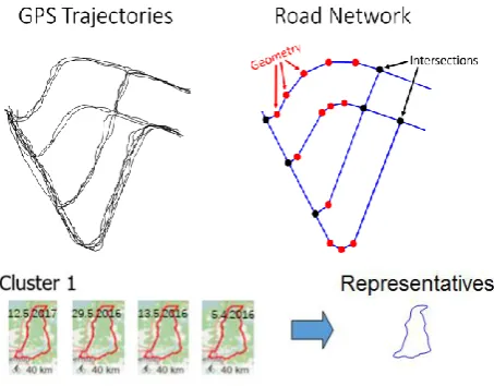
We study the problem of finding a good representative of a set of GPS trajectories. Solutions are needed in several applications such as extracting road network, trajectory clustering, and calculating average routes for taxi trips, see Figure 1. The input is an ordered sequence of geographical points (latitude, longitude), and the output is a polygon that approximates the path traveled.
Figure 1. Averaging a set of GPS trajectories is needed in road network extraction (above) and clustering of GPS trajectories (below).
The problem is closely related to averaging of time series, which has been studied actively in recent years in the context of dynamic time warping (DTW) distance. The common problem is that the observations may have collected with different frequency, and the number of samples varies across the sequences. The major issue is how to align the sequences before the averaging. Earlier studies have considered the problem as multiple sequence alignment (MSA), which is equivalent to the Steiner sequence [1]. However, it was recently shown that the multiple alignment approach does not guarantee optimality [2].
It is possible to solve the averaging problem by using Mean, which is defined as any sequence that minimizes the sum of squared distances to all the input sequences:
(
)
=
k
i i
C D x C
1
2
, min
arg (1)
where X={x1, x2, …, xk} is the set of input sequences, and C is the mean. This definition defines averaging nicely as an optimization problem. However, the search space is huge, and exhaustive search by enumeration is not feasible. Exponential time algorithm for solving the exact DTW-mean was recently given in [2], but the problem was shown to be NP-hard concerning the number of sequences [3].
The GPS trajectories differ from time series in a few ways. First, the alignment of the time series is performed in the time domain while the GPS points need to be aligned in geographical space. Second, GPS data can be noisy. This means that the mean might not even be the best solution to the problem.
The averaging problem of GPS trajectories has been recently studied in a Segment averaging challenge1 2019 with several new solutions proposed [4]. Most methods in the competition apply the four-step procedure shown in Figure 2. Some trajectories can be stored in reverse order, and re-ordering of the sequences is needed. Outlier removal is commonly applied to reduce the effect of the noisy trajectories. After these steps, the problem reduces to normal sequence averaging. Post-processing by polygonal approximation is sometimes also done to simplify the final representation.
Sequence averaging
Re-ordering removalOutlier approximationPolygonal
Figure 2. Collection of raw GPS trajectories (left), and extracted road network (right).
Although several reasonable solutions have been proposed, several of them are rather complicated, and some also suffer from high time complexity. In this paper, we present three rapid and simple methods based on analyzing three descriptors of the curves: start (S), middle (M), and destination (D), see Figure 3. If the trajectory resembles a line, a simple linear model with 2 or 3 points is produced. Otherwise, a more complex curvy model is applied as a back-up. Three methods are considered for this: Median, Medoid, and Divide-and-Conquer.
The rest of the paper is organized as follows. Existing methods are reviewed in Section 2. The three proposed methods are introduced in Section 3. Experiments are performed in Section 4, and conclusions are drawn in Section 5.
Figure 3. Sketch of the proposed solution: trajectories are analyzed based on three descriptors: start (S), middle (M), and destination (D).
2. Existing works on segment averaging
In [5], average segments (called centreline) were used for k-means clustering of the GPS trajectories to detect road lanes. The averaging method was later defined in [6] based on piecewise linear regression. The data is treated as an unordered set of points for which piecewise polynomials are fit with continuity conditions at the knot points [7]. The drawback of using regression is that we lose the information in which order points were collected, which makes the problem harder to solve. In the Segment averaging challenge [4], only one proposal was based on the regression approach, and its performance was not among the best.
Recent solutions consider the problem as sequence averaging and apply methods from time series context using dynamic time warping as distance function. For example, the CellNet segment averaging [8] takes the shortest path as the initial guess [9] and then applies the Majorize-minimize iterative algorithm [1] to estimate the mean. Another iterative algorithm uses kernelized time elastic averaging (iTEKA) for the averaging [10]. It considers all possible alignment paths and integrates a forward and backward alignment principle jointly.
Medoid is an alternative approach to mean. It is also defined as an optimization problem but with the difference that, instead of allowing any sequence, Medoid is selected as one of the input sequences. The problem can then be solved brute force by calculating all pairwise distances and selecting the sequence that minimizes the optimization function. Possible functions to measure the distance (or similarity) between GPS trajectories have been extensively studied in [11] and tested with the Medoid in [4]. In this paper, we use Hausdorff distance [12] as it is invariant to the travel order of the trajectories, and it provides competitive results among the other choices.
Medoid has two main drawbacks. First, it requires O(k2) distance calculations, where k is the number of trajectories. Standard implementations of distance functions like dynamic time warping usually require O(n2) where n is the number of points in the longest trajectory. Thus, the total time complexity can be as high as O(k2n2). Another drawback is that Medoid is limited to be one of the input trajectories, which can be a poor approximation of the average segment, especially if k is small.
3. Three rapid methods
We next present three new methods for solving the problem:
• RapSeg-A: Median for curvy segments
• RapSeg-B: Medoid for curvy segments
• RapSeg-C: Divide-and-conquer approach
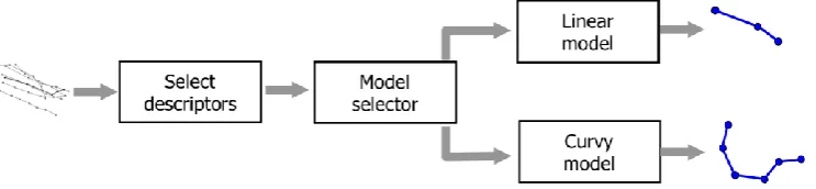
All methods use the same overall structure, as shown in Figure 4. Three descriptors are first calculated to describe the set of trajectories. Based on these descriptors, we estimate whether a simple linear model can describe the set or a more complex model is necessary. We design two alternative models for these: the linear model and the curvy model.
Figure 4. The general structure of the three methods.
3.1. Descriptors and model selector
invariant to the travel direction, the order of S and D can be chosen arbitrarily. Next, we analyze the trajectories and select the median (middle point) from every trajectory to get median set. Finally, we calculate the average (centroid) of each of those three sets to produce the triple (S, M, D). The process is summarized in Figure 5.
Figure 5. Flow diagram of selecting the three descriptors.
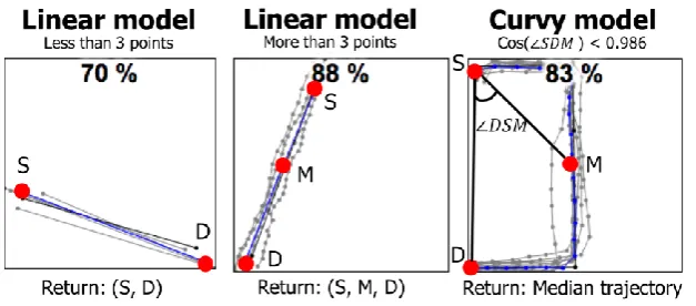
The descriptors are then used to decide whether the set can be described by a linear model. We compare the straight line SD against the two-segment line SMD, which makes detour via the median point M. The more the detour deviates from the direct connection, the less likely a simple linear model is suitable to describe the segment. The exact criterion is the angle: SDM and DSM. If the cosine of the angle is less than a threshold (0.986), we use a curvy model. We call the method as Rapid Segment (RapSeg), see Algorithm 1 and Figure 3.
Algorithm 1:RapSeg(X, threshold): S, M, D LineSegment(X);
IF cos(SDM) threshold || cos(DSM) threshold: RETURN CurveSegment(X);
ELSE:
RETURN S, M, D;
Examples of sets and their descriptors are shown in Figure 6. The first four examples have an only slight change of direction, and the linear model is therefore applied. The four examples below did not meet the angle criterion, and curvy model is applied. Examples are shown using the median segment.
3.2. Linear model
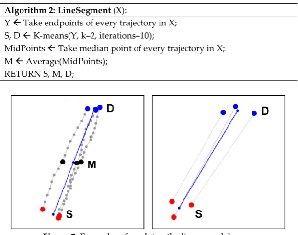
Our linear model is straightforward. We use the triple (S, M, D) as a three-point model to represent the segment. Only in the case when all trajectories have only two points, we output (S, D) as the model. Algorithm 2 details the process, and examples are shown in Figure 7.
Algorithm 2:LineSegment (X):
Y Take endpoints of every trajectory in X; S, D K-means(Y, k=2, iterations=10);
MidPoints Take median point of every trajectory in X; M Average(MidPoints);
RETURN S, M, D;
Figure 7. Examples of applying the linear model.
3.3. Curvy model A: Median
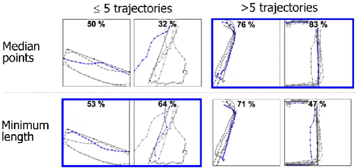
As a back-up strategy, we select one of the input trajectories to represent the segment. To keep the method simple, we calculate the number of points in the trajectories and select the trajectory with the median number, shown in Algorithm 3. We also considered the alternative strategy used in [8, 9], which selects the trajectory with the shortest path length. It sometimes works better, especially when there are only a few trajectories in the set, but it has problems when there are more trajectories in the set, see Figure 8. For simplicity, we stick to the median points strategy.
Algorithm 3 (RapSeg-A): CurveSegment (X): FOR every trajectory Xi:
Ni Calculate the number of points in Xi;
Figure 8. Examples of curved sets. The trajectories of minimum length and the median number of points are considered as representatives.
3.4. Curvy model B: Medoid
The previous model is highly heuristic, and a more systematic choice can be made. Medoid is defined as the sample whose total distance to all other samples is minimal, shown in Eq. (2). This can also be applied to the segment averaging problem if we define suitable distance function between the GPS trajectories, shown in Algorithm 4. We use Hausdorff [12] as it is invariant to the travel distance and produces competitive results. Potentially better choices could be found in [11] but since Medoid is not the main strategy we settle with Hausdorff distance.
Algorithm 4 (RapSeg-B): CurveSegment (X): j find the medoid from X via Eq. (2) RETURN Xj;
In the context of GPS trajectories, we define Medoid as the input sequence xj that minimizes the following function:
(2)
The downside of the Medoid is its higher time complexity. Assuming that there are k trajectories to consider, each having at most n points. The time complexity of single Hausdorff computation takes O(n2) so the total time complexity of finding the Medoid is O(k2n2). It is possible to use faster distance measures like Euclidean and Fast-DTW [13], but issues like having trajectories of different lengths and different point orders can have unwanted effects. In addition, linking components from multiple libraries can easily cancel the effect of an otherwise good idea – as also happened in [8]. We, therefore, settle here with the standard Hausdorff function:
=
) , (
) , ( max ) , Hausdorff(
A B d
B A d B
A (3)
where A and B are the two trajectories and dist is the Euclidean distance between two points.
3.5. Curvy model C: divide-and-conquer
at the median points (M) of each trajectory. Both sub-segments are then recursively processed by the same overall algorithm until the sub-segment reduces to the linear model. See Algorithm 5 and Figure 9.
Algorithm 5 (RapSeg-C): CurveSegment (X, S, D, threshold):
M calculate the mean of the set of median points from each trajectory in X; IF cos(SDM) threshold || cos(DSM) threshold:
X1, X2 cut each trajectory in X into two parts by the point at the median location; CurveSegment (X1, S, M, T);
CurveSegment (X2, M, D, T); ELSE:
RETURN M;
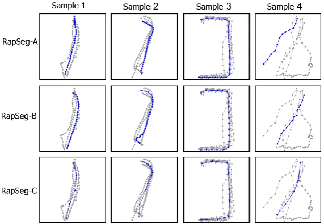
An example of this curvy model is shown in Figure 9. We notice how the shape depicted by the set of trajectories is preserved. Figure 10 shows that in comparison with the methods A and B, the resulting segment produced by Variant C has much fewer points and generally looks better upon visual inspection.
Figure 9. Examples of divide-and-conquer (RapSeg-C) approach for handling the curvy model.
3.6. Outlier removal
The data contains many noisy trajectories. We, therefore, consider detecting and removing outliers as a pre-processing step. For simplicity, we apply an existing generic outlier detection method called Local outlier factor (LOF) [14] (See Figure 11). It calculates the local density for every point as the distance to its furthest k nearest neighbor. Points having a significantly lower density than their neighbors, are more likely to be outliers. The outlierness of a point is the ratio of its density relative to the density of its neighbors. We apply LOF separately to source destination sets, and detect top-10% outlier points. A trajectory is removed if either their start or end point is detected as an outlier.
Figure 11. Outlier removal.
We smooth the effect of the outlier removal as follows. We calculate the descriptors (S, M, D) for the set both with (variant 1) and without (variant 2) outlier removal as illustrated in Algorithm 6. The final descriptors are then weighted averages of the two alternatives. We experimentally select the weights as a=0.016, b=0.600, c=0.510.
Algorithm 6: Embedding (variant 1, variant 2) a, b, c = 0.016, 0.600, 0.510;
IF SIZE (variant 2)>3: RETURN variant 2; ELSE:
S1, M1, D1 variant 1; S2, M2, D2 variant 2;
IF SIZE(M2)==0 : // M2 is empty
S = 2*a*S1+(1+a)*S2; D = 2*a*D1+(1+a)*D2; RETURN S, D; ELSE:
RETURN S2, (b* M2+(1-b)*(c* S2+(1-c)* D2)), D2;
3.7. Time complexity
Table 1. The time complexity of the proposed methods.
Step Solution Complexity
Linear Segment
Endpoints Table look-up O(k)
K-means Clustering O(k)1
Median points Table look-up + average O(k)
Curve Segment
RapSeg-A: Median Selection O(k)
RapSeg-B: Medoid Hausdorff O(n2k2)
RapSeg-C: Divide-and-Conquer Calculate M O(Tk) 1 Assuming 10 iterations of k-means with 2 clusters: 210k = 20k = O(k)
4. Experiments
We use the datasets described in [4], which is also found via the following web site:
http://cs.uef.fi/sipu/segments. The data include intersections taken from the open street map (OSM), and trajectories between those intersections, selected from four different data collections: Joensuu 2015 [15], Chicago [16], Berlin [17], and Athens [17]. The sets were grouped together and then randomly divided into 10% for training (100 sets) and 90% for testing (901 sets). There are a total of 10,480 trajectories consisting of 90,231 points. More details of the data extraction are available in [4].
For evaluating the accuracy of the segments, we use hierarchical cell-based similarity measure (HC-SIM) as proposed in [4]. It extends C-SIM measure2 [15] to multiple zoom levels. C-SIM uses a grid of 2525 meters and counts how many cells the resulting segment average share with the ground truth segments from OSM relative to the total number of cells they occupy. HC-SIM uses six layers with the following grid sizes: 2525m, 5050m, 100100m, 200200m, 400400m 800800m. In case of the [0, 1] scale, the following sizes are used: 0.5%, 1%, 2%, 4%, 8%, 16%.
4.2. Results
The effect of the threshold is shown in Figure 12. The results show that we can achieve good results even with the linear model. For example, RapSeg-A reaches 62.0% even without the curvy model. We set the threshold to 0.986 based on the training as the performance seems to peek at that point. RapSeg-C reaches the best performance of 62.2%. If the threshold was increased further, the maximum performance of 62.3% could have been reached. Most of the performance is achieved already by the linear model, which indicates unbalance of the line and curve shapes in the dataset.
Figure 12. Effect of the threshold. The higher the value, the more often the curvy model is used.
The effect of outlier removal is shown in Table 2. It clearly improves the performance with the training data, and the smoothed variant is always better than the full outlier removal as such. However, the results do not generalize to the test data, and the best results are reached by RapSeg-A and RapSeg-C without any outlier removal step at all. We, therefore, drop the outlier removal from the final method completely.
Table 2. Effect of outlier removal on the three variants.
Outlier removal RapSeg-A RapSeg-B RapSeg-C
Tra
in --- 67.4 % 68.3 % 67.9 %
Smoothed 69.4 % 70.2 % 69.5 %
Full 69.0 % 69.7 % 69.3 %
Te
st --- 62.0 % 61.9 % 62.2 %
Smoothed 61.8 % 61.9 % 62.0 %
Full 61.3 % 61.4 % 61.5 %
Comparison of the RapSeg method (without the outlier removal) is compared against existing techniques in Table 3. All variants outperform the existing methods on accuracy, processing time and the number of points. In other words, RapSeg does not only provide more accurate approximation of the segment but it also save processing time. Closest competitor in terms of accuracy is the method by Marteau [18].
The performance of the different curve models are compared in Table 4. We can see that RapSeg-A has the best performance of length and processing time, while RapSeg-C has the best performance on accuracy and the number of points. Their main difference is the processing time; RapSeg-B takes 5 times longer than RapSeg-A (0.59s vs. 3.39s) while RapSeg–C is almost as efficient (0.56s vs. 0.67s). From the visual examples in Figure 13, we can see that all method provide satisfactory results whereas RapSeg-A appears to be more robust on noise.
Table 3. Comparison of the methods. Length and points are given relative to the corresponding numbers in the ground truth; so 100% denotes the expected result.
Method Accuracy Length Points Time
Medoid [4] 56.40% 98% 169% ~1 hour
CellNet [8] 53.80% 65% 144% 49 s
CellNeto [8] 61.20% 96% 144% 48 s
Marteau [18] 61.70% 99% 145% 30 min
RapSeg-A 62.00% 99% 81% 12 s
RapSeg-B 62.10% 99% 79% 16 s
RapSeg-C 62.20% 99% 77% 13 s
Table 4. Comparison of the proposed methods on curve model.
Method Accuracy Length Points Time
RapSeg-A 53.05% 99% 194% 0.59 s
RapSeg-B 53.26% 89% 167% 3.39 s
RapSeg-C 55.53% 95% 120% 0.67 s
Further analysis by calculating Spearman correlation showed that the performance of RapSeg (all variants) correlates with the number of points (0.19 – 0.34), and with the number of trajectories (0.22 – 0.25). A positive correlation is expected as more samples are expected to provide a better chance to derive the correct segment from the data. On the testing data, a negative correlation was observed between the performance and the variance3 between the trajectories in the set (-0.25). This is also as expected because it should be easier to find the correct segment average for a set with tighter packed trajectories. However, there is no correlation on the training set (0.06 Spearman correlation), which may be explained by the fact that the training set is smaller and populated by many sets containing only a few sample trajectories which can skew the numbers.
Figure 13. Visualizations of the three methods for handling the curvy model on samples in the test dataset.
5. Conclusions
Three fast segment averaging methods were proposed to handle complex curve segments. The results showed that the simplest variant (RapSeg-A) achieves virtually as good accuracy as the more complex variant (RapSeg-C); 62.0% vs. 62.2%. All methods are fast, simple to implement, and do not suffer serious over-sampling.
References
1. Hautamäki V., Nykänen P., Fränti P. Time-series clustering by approximate prototypes, Int. Conf. on Pattern Recognition, pp. 1-4, 2008.
2. Brill M., Fluschnik T., Froese V., Jain B. Niedermeier R., Schultz D., Exact mean computation in dynamic time warping spaces, Data Mining, and Knowledge Discovery, 33: 252–291, 2019.
3. Bulteau L., Froese V., Niedermeier R. Tight hardness results for consensus problems on circular strings,
ArXiv 1804.02854-v4, 2019.
4. Fränti, P. and Mariescu-Istodor, R. Averaging GPS segments challenge 2019. Manuscript (under preparation).
5. Wagstaff K., Cardie C., Rogers S., and Schrödl S. Constrained k-means clustering with background knowledge. Int. Conf. on Machine Learning (ICML '01), 577-584, 2001.
6. Schroedl S., Wagstaff K., Rogers S., Langley P., Wilson C. Mining GPS traces for map refinement, Data Mining and Knowledge Discovery, 59-87, 2004.
7. Piegl L. and Tiller W. The NURBS Book (2nd Ed.). Springer-Verlag, 1997.
8. Mariescu-Istodor R. and Fränti P. Cellnet: Inferring road networks from GPS trajectories. ACM Transactions on Spatial Algorithms and Systems 4 (3), 2018.
10. Marteau P.-F., Times series averaging and denoising from a probabilistic perspective on time-elastic kernels, Int. J. Applied Mathematics and Computer Science, 29 (2), 2019.
11. Mariescu-Istodor R. and Fränti P. Grid-based method for GPS route analysis for retrieval, ACM Transactions on Spatial Algorithms and Systems 3 (3), 2017.
12. Rockafellar T.R. and Wets R.J.-B. Variational analysis, Springer Science & Business Media, 317, 2009. 13. Salvador S. and Chan P. Toward accurate dynamic time warping in linear time and space, ACM Int.
Conf. on Knowledge Discovery and Data Mining Workshop on Mining Temporal and Sequential Data, pp. 70– 80, 2007.
14. Breunig M.M., Kriegel H., Ng R.T., and Sander J. LOF: Identifying density-based local outliers, ACM SIGMOD Int. Conf. on Management of Data, 29 (2), 93-104, 2000.
15. Mariescu-Istodor R. and Fränti P. Grid-based method for GPS route analysis for retrieval, ACM Transactions on Spatial Algorithms and Systems 3 (3), 2017.
16. Biagioni T. and Eriksson J. Inferring road maps from global positioning system traces: Survey and comparative evaluation. Transportation Research Record: Journal of the Transportation Research Board, 61-71, 2012.
17. Ahmed M., Karagiorgou S., Pfoser D., and Wenk C. A comparison and evaluation of map construction algorithms. GeoInformatica, 601-632, 2015.