Limit Load Analysis Using the Reference Volume Concept

Limit Load Analysis Using the Reference Volume Concept

Ihab F. Z. Fanous1,2 and R. Seshadri1

1. Faculty of Engineering and Applied Science, Memorial University of Newfoundland, St. John's, NL, Canada 2. Currently at Atomic Energy of Canada Limited (AECL), Mississauga, ON, Canada

ABSTRACT

Limit load analysis is usually performed by the interpretation of stress redistribution using either linear elastic or inelastic methods. Several redistribution iterations are required to achieve an accurate estimate of the limit load. In this paper the reference volume method is illustrated and shown to be effective in finding the limit load using few linear elastic redistribution iterations. The reference volume is based on the concept of using a part of the volume of the component that is undergoing plastic deformation. The method is applied to a number of problems illustrating different cases of reference volumes to verify the analysis procedure.

INTRODUCTION

The limit load is an essential tool for the integrity assessment of pressure components. Analytical methods have been developed for simple components. Elastic-plastic analysis is widely used in complex problems for evaluation of limit load. In performing and elastic-plastic finite element analysis, the load is increased incrementally until a further incremental loading would cause unstable behavior. Different criteria are defined to interpret their results to estimate the limit load. One of these criteria, as defined by the ASME, is the twice the elastic slope. However, the non-linear methods for stress analysis have a lot of complexities. Therefore, robust methods are desirable in order to simplify the stress analysis procedure and limit load estimation. The Elastic Modulus Adjustment Procedure (EMAP) [1] was developed in which elastic analysis is used to find the inelastic stress distribution due to an applied state of loading. The method was used mainly for the estimation of the limit load. The GLOSS method [2] was also developed utilizing the elastic modulus modification concept to find the stress redistribution due to multi-axial creep relaxation. Hence, the stress distribution can be used to calculate the reference stress, which inturn can be used to calculate the lower bound limit load.

CLASSICAL LIMIT LOAD MULTIPLIER

The classical upper bound solution is based on the comparison of the response of an assumed solution to a postulated collapse mechanism achieved by a kinematically admissible solution. Considering a body subjected to some distribution of tractions T, the factor m by which the loading can be increased before the solid collapses (m is effectively the factor of safety) is estimated. It is assumed that the component will collapse when subjected to loading mT. Assuming

ij

s is the deviatoric stress of the exact solution and ε_&ij is a kinematically admissible solution for the given problem, it can be deduced using Schwartz’s inequality that

0 p p

ij ij ij ij ij ij sε s s ε ε

≤ & ≤ & & (1)

On the basis that σy= 3s sij ij 2 for the exact solution, equation (1) becomes

2 3

p p p

ij ij y ij ij y e

sε& ≤ σ ε ε& & =σ ε& (2)

Using the principle of virtual work and integrating on both sides gives

0

F y e i i

V S

dV mT u dA

σ ε − ≥

∫

∫

Assuming an elastic stress field *

ij

*

0

F

p

ij ij i i

V S

s ε dV− T u dA=

∫

∫

Substituting equation (4) into equation (3) gives

*

0

p p

y ij ij ij

V V

dV m s dV

σ ε − ε ≥

∫

∫

Rearranging gives * y e V u p ij ij V dV m m s dV σ ε ε ≤

∫

∫

& (6)

This equation is translated to the finite elements form as

1

1 N

ek k k u y N

ek ek k k V m V ε σ σ ε = = =

∑

∑

THEORY

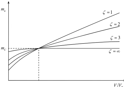
Seshadri and Mangalaramanan [3] have observed that, if plastic collapse occurs over a localized region of the mechanical component or structure, the upper bound multiplier will be significantly overestimated if it is calculated on the basis of the total volume, VT. Furthermore, the corresponding mL, which is calculated based on a single element that has the maximum equivalent stress in the component, will be underestimated. During local collapse, plastic action is confined to a sub-region of the total volume, and the remainder region, remains unchanged and, thus, the strain rate will be zero. Hence, the magnitude of the upper bound multiplier (m_u) would depend on the sub-volume, V_β, where

(

)

=

∑

within which the elements are arranged in the order of

1 2

e e eβ

σ >σ >L>σ (9)

Eliminating the part of the volume with zero strain rate in equation (6) of the, the upper bound multiplier becomes dependant on the reference volume V_R and is expressed as

( )

R

y e V

u R _p

ij ij V

dV

m V m s dV σ ε ε =

∫

∫

& (10)

In addition, for an infinitesimally small value of * V , *

ij

s will be at the highly stressed point in the component and the

calculated multiplier becomes the classical lower bound solution mL. The variation of mu and mL with the redistribution of

Fig. 1: Variation of mu and mL with iteration of stress redistribution

Hence, in terms of finite elements, the multiplier will be

1

1 R

R N

ek k k u y N

ek ek k k

V m

V ε σ

σ ε

=

=

=

∑

∑

where NR is the number of elements in the reference volume.

To find the reference volume, the elements are sorted according to equation (9) and mu is calculated using equation

(11) starting with N_R=1 (single element) until N_R =N_T (total volume). This is done for every iteration and m_u is plotted versus the considered volume as shown in Fig. 2. The intersecting point between iteration ζ and ζ+1 will be the solution for iteration ζ+1.

C m

T V V 1

ζ =

2

ζ =

3

ζ =

ζ = ∞

u m

C m

ζ u

m m Vu

( )

( )

( )

u R m V

( )

APPLICATIONS

Indeterminate beam

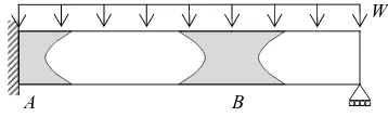
The indeterminate beam is selected to illustrate the reference volume analysis because it is known from previous work that it fails by the formation of two plastic hinges within confined regions. Also, the problem is solved analytically by Mendelson [4]. At the state of collapse, the plastic hinges are formed at locations A and B shown in Fig. 3. Hence, the regions of the hinges have stresses in the plastic range while the rest of the beam will have a near zero stress distribution.

Fig. 3: Schematic diagram of the indeterminate beam.

The length of the beam is 0.508 m with 2.54 cm height and width. The material used has an elastic modulus of 206.8 MPa. The beam is modeled as plane stress and solved using ABAQUS [5]. The redistribution of the stresses is introduced into ABAQUS using the user-subroutine feature UMAT to define a non-standard material behavior. In the sub-routine, the equations of the elastic behavior is developed while adjusting the elastic modulus for using the calculated stress fields. Using the results of the stress redistribution analysis, the elements are sorted according to equation (9). Hence, the upper bound multiplier is calculate based on several selected partial volumes V_P using the equation

P

P

e V

u y p

ij ij V

dV

m

s dV ε σ

ε

=

∫

∫

&

& (12)

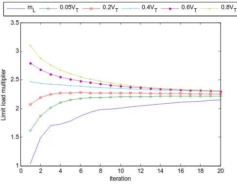
for different ratios of V V_{P T} . Figure 4 shows a plot of the calculated values of the multiplier versus the iteration variable. It can be noticed that the curve tends to flatten to a constant value as the volume decrease to a value just below 40% of the total volume. By comparing the first two iterations of the analysis, the reference volume was found to be that which is defined by the stress greater than 51.1 MPa illustrated in Fig. 5 which was found to be 34.5% of the total volume. Also, the value of the multiplier approach the classical lower bound as the partial volume tends to the minimum value, which is the volume of the element having the highest stress.

W

0 2 4 6 8 10 12 14 16 18 20 1

1.5 2 2.5 3 3.5

Iteration

Li

m

it

l

oad

m

ul

ti

pl

ier

m_L 0.05V_T 0.2V_T 0.4V_T 0.6V_T 0.8V_T

Fig. 4: The upper bound multiplier for selected partial volumes.

Figure 6 shows the results of the analysis comparing the classical upper bound, classical lower bound, r-node and reference volume solutions. It can be observed how the multiplier calculated using the reference volume converged as an upper bound solution faster than the other methods.

Fig. 5: Reference volume of the indeterminate beam.

0 2 4 6 8 10 12 14 16 18 20 1

1.5 2 2.5 3 3.5

Iteration

Li

m

it

l

oad m

ul

ti

pl

ier

Oblique nozzle

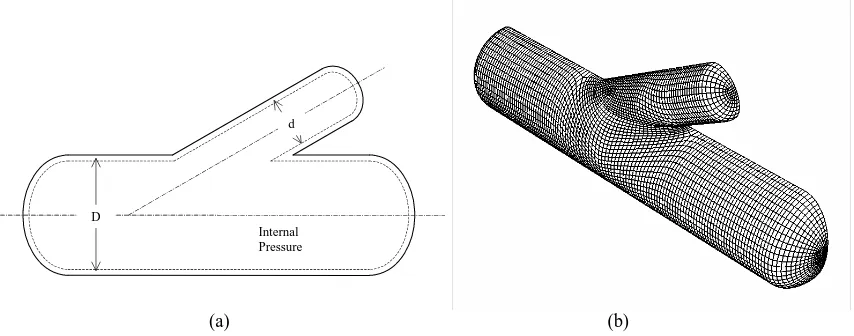
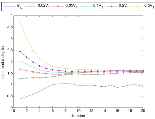
A complex problem that has been considered in many investigations is the analysis of an oblique nozzle attached to a pressure vessel as shown in Fig. 7(a). Sang et al [6] has conducted a set of experiments and elastic-plastic finite element analysis to monitor the complete stress distribution and find the limit load of the problem. The reference volume procedure is applied to the oblique nozzle presented by Sang et al [6] to compare its results with the experimental values. Also, the limit load is calculated using the upper bound multiplier, the classical lower bound multiplier and the r-node analysis to observe the convergence of the reference volume.

The inside diameter and thickness of the vessel are 600 mm and 6 mm, respectively. The outside diameter and thickness of the nozzle are 325 mm and 6 mm, respectively. The oblique angle is 30º. The length of the shell is 2400 mm and the length of the nozzle is 600 mm. The finite element model is done using 4-noded layered shell elements with 20 layers. Fig. 7(b) shows the meshing of the described geometry. Half of the geometry is being considered making use of the symmetrical characteristic.

Internal Pressure D

d

(a) (b)

Fig. 7: (a) Schematic diagram of the cross-section of an oblique nozzle used for experimental analysis by Sang et. al [6]. (b) Suggested meshing of the geometry.

0 2 4 6 8 10 12 14 16 18 20 0

0.5 1 1.5 2 2.5 3 3.5 4

Iteration

Li

m

it

l

oad

m

ul

ti

pl

ier

m_L 0.02V_T 0.05V_T 0.1V_T 0.2V_T 0.5V_T

Fig. 8: Upper bound multiplier based on partial volumes.

0 2 4 6 8 10 12 14 16 18 20 0

0.5 1 1.5 2 2.5 3 3.5 4

Iteration

Li

m

it

l

oad

m

ul

ti

pl

ier

Experimental R-Node m_c m_u m_v

Fig. 9: Upper bound multiplier based on partial volumes.

CONCLUSION

The limit load analysis using the finite element method requires several stress redistribution analysis, especially with highly complex problems. Using the fact that only part of the structure undergoes plastic deformation, the concept of the reference volume is introduced in which the upper-bound limit load multiplier is calculated based on part of the total volume. Comparing the variation of the upper-bound multiplier for two linear elastic analyses with increasing volume starting with the elements having the highest centroid stress gives the volume at which the multiplier remains constant and this is set as the reference volume. The results of the reference volume analysis method compares well with the analytical and experimental solutions of several problems with reasonable accuracy and convergence rate. It can be used to calculate the limit load using two or thee elastic iterations.

REFERENCES

[1] Mackenzie, D., and Boyle, J. T., 1993, ‘‘A Method of Estimating Limit Loads by Iterative Elastic Analysis I: Simple

Examples,’’ Int. J. Pressure Vessels Piping, 53, pp. 77–95.

[2] Seshadri, R., "The Generalized Local Stress Strain (GLOSS) Analysis—Theory and Applications," ASME J.

Pressure Vessel Technol., 113, 1991, pp. 219–227.

[3] Mangalaramanan, S. P., and Seshadri, R., ‘‘Limit Loads of Layered Beams and Layered Cylindrical Shells using

Reduced Modulus Methods,’’ ASME Pressure Vessels and Piping Conference, 1997, Orlando, FL.

[4] Mendelson, Alexander, 1968, Plasticity: Theory and Application, The MacMillan Company, NY.

[5] Hibbitt, Karlsson, and Sorensen, ‘‘ABAQUS/Standard User’s Manual,’’ 6.2, 2001.

[6] Sang, Z. F., Y. J. Lin, L. P. Xue and G. E. O, Widera, “Limit and Burst Pressures for a Cylindrical Vessel With a 30