Stability analysis of shallow undrained tunnel heading using finite element limit analysis

(1)

ii

University of Southern Queensland

Faculty of Health, Engineering & Sciences

STABILITY ANALYSIS OF SHALLOW

UNDRAINED TUNNEL HEADING USING

FINITE ELEMENT LIMIT ANALYSIS

A dissertation submitted by

Mr. Alexander Bell

In fulfilment of the requirements of

Bachelor of Engineering (Civil)

(2)

i

ABSTRACT

This dissertation investigated the undrained stability of shallow tunnel heading problems subjected to varying loading conditions by performing a two-dimensional plane strain analysis. Failure due to the blowout mechanism was highlighted as a major focus area, due to the lack of previous research on the topic. Finite element limit analysis (FELA), employed through the geotechnical software analysis package, Optum G2, was used to determine lower and upper bound factor of safety (FoS) values for a range of various scenarios. The factor of safety values were calculated using the gravity multiplier method (GMM) and the strength reduction method (SRM). These methods were directly compared and the strength reduction method was found to be the most suitable method for analysing scenarios with either a surcharge or internal tunnel pressure applied. The results obtained in this study were validated by comparing a sample to results published by Augarde, Lyamin and Sloan (2003). This comparison found a very good level of agreement.

The factor of safety is a function of three dimensionless parameters; the pressure ratio (PR), strength ratio (SR) and depth ratio (DR). The relationship between the factor of safety and these parameters was investigated. A number of plots and displacement vector fields were created to better assist in understanding these relationships and the specific failure mechanism related to each scenario. This process reinforced the need to not only design tunnels for failure due to collapse but to also check for failure due to blowout.

(3)

ii

DISCLAIMER PAGE

University of Southern Queensland

Faculty of Health, Engineering and Sciences

ENG411/ENG4112 Research Project

Limitations of Use

The Council of the University of Southern Queensland, its Faculty of Health, Engineering & Sciences, and the staff of the University of Southern Queensland, do not accept any responsibility for the truth, accuracy, or completeness of material contained within or associated with this dissertation.

Persons using all or any part of this material do so at their own risk, and not at the risk of the Council of the University of Southern Queensland, its Faculty of Health, Engineering & Sciences or the staff of the University of Southern Queensland.

(4)

iii

CANDIDATE’S CERTIFICATION

University of Southern Queensland

Faculty of Health, Engineering & Sciences

ENG4111/ENG4112 Research Project

Certification of Dissertation

I certify that the ideas, designs and experimental work, results, analyses and conclusions set out in this dissertation are entirely my own effort except where otherwise indicated and acknowledged.

I further certify that the work is original and has not been previously submitted for assessment in any other course or institution, except where specifically stated.

(5)

iv

ACKNOWLEDGEMENTS

(6)

v

1

TABLE OF CONTENTS

ABSTRACT ... i

DISCLAIMER PAGE ... ii

CANDIDATE’S CERTIFICATION ... iii

ACKNOWLEDGEMENTS ... iv

TABLE OF FIGURES ... viii

TABLE OF TABLES ... xiii

CHAPTER 1: INTRODUCTION ... 1

1.1 Outline of Study ... 1

1.2 Methodology ... 2

1.3 Research Objectives ... 3

1.4 Organisation of Thesis ... 3

CHAPTER 2: GENERAL REVIEW ... 6

2.1 Introduction ... 6

2.2 Significance of Tunnels... 6

2.3 Tunnelling Terminology ... 7

2.4 History of Tunnels ... 7

2.5 Tunnel Construction Methods ... 11

2.6 Design Criteria ... 15

2.7 Tunnel Stability Review ... 16

2.8 Factor of Safety Approach ... 20

CHAPTER 3: NUMERICAL MODELLING REVIEW ... 23

3.1 Optum G2 Introduction ... 23

3.2 Finite Element Limit Analysis ... 23

3.3 Gravity Multiplier Method ... 24

3.4 Strength Reduction Method ... 25

(7)

vi

3.6 Optum G2 Slope Example ... 30

3.7 Optum G2 Tunnel Heading Example ... 34

CHAPTER 4: TUNNEL HEADING ANALYSIS: COLLAPSE ... 41

4.2 Problem Statement ... 41

4.3 2D Tunnel Heading Numerical Modelling... 45

4.4 Factor of Safety Bounds ... 46

4.5 Internal Comparison of Collapse Results ... 48

4.6 External Comparison of Collapse Results ... 55

4.7 Optum G2 Tunnel Heading Collapse Results and Discussion ... 57

4.8 Conclusion ... 66

CHAPTER 5: TUNNEL HEADING ANALYSIS: BLOWOUT ... 68

5.3 Significance of the Blowout Failure Mechanism ... 72

5.4 2D Tunnel heading Numerical Modelling ... 73

5.6 Internal Comparison of Blowout Results ... 76

5.7 Optum G2 Tunnel Heading Blowout Results and Discussion ... 82

CHAPTER 6: TUNNEL HEADING ANALYSIS: STABILITY DESIGN CHARTS ... 93

6.3 2D Tunnel Heading Numerical Modelling... 96

6.5 Optum G2 Tunnel Heading Results and Discussion ... 99

6.6 Tunnel Heading Stability Design Charts ... 103

(8)

vii

CHAPTER 7: CONCLUSION ... 114

7.1 Summary ... 114

7.2 Future Research ... 116

REFERENCES ... 117

APPENDIX A – PROJECT SPECIFICATION ... 121

APPENDIX B – INITIAL RESULTS AND PLOTS ... 122

APPENDIX C – EXTERNAL COMPARISON ... 131

(9)

viii

TABLE OF FIGURES

(10)

ix

(11)

x

Figure 3.23: Upper bound SRM results of tunnel heading example showing σ1, σ2 vectors

(Optum Computational Engineering 2016). ... 39

Figure 3.24: Upper bound SRM results of tunnel heading example showing plastic multiplier (Optum Computational Engineering 2016). ... 40

Figure 4.1: Tunnel heading stability problem statement. ... 42

Figure 4.2: Example of collapse failure mechanism produced in Optum G2 showing plastic multiplier and 60% deformation scale. DR = 2, SR = 1.10, PR = +10. ... 45

Figure 4.3: Tunnel heading finite element mesh with mesh adaptivity. ... 46

Figure 4.4: Graphical comparison of upper and lower bound results obtained through SRM for PR = 0. ... 49

Figure 4.5: Graphical comparison of upper and lower bound results obtained through GMM for PR = 0. ... 49

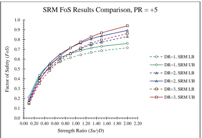
Figure 4.6: Graphical comparison of upper and lower bound results obtained through SRM for PR = +5. ... 54

Figure 4.7: Comparison of collapse results to external publication. [1] Denotes data obtained from Augarde, Lyamin and Sloan (2003)... 56

Figure 4.8: Tunnel heading failure by collapse showing displacement vector field and mesh overlay. PR=0, DR=2 & SR=1.50. ... 58

Figure 4.9: Plot of factor of safety verse pressure ratio for tunnel heading problem, DR = 2 and SR = 1.50. ... 59

Figure 4.10: Displacement vector field. PR = +10, DR = 2, SR = 1.50. ... 60

Figure 4.14: Displacement vector field. PR = 0, DR = 2, SR = 1.50. ... 61

Figure 4.15: Displacement vector field. PR = -1, DR = 2, SR = 1.50. ... 61

Figure 4.16: Displacement vector field. PR = -1.5, DR = 2, SR = 1.50. ... 62

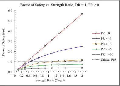
Figure 4.17: Factor of safety vs. strength ratio for all positive pressure ratios. DR = 1. . 63

Figure 4.18: Factor of safety vs. strength ratio for all positive pressure ratios. DR = 2. . 63

(12)

xi

Figure 5.2: Example of blowout failure mechanism produced in Optum G2 showing plastic multiplier and 60% deformation scale. DR = 2, SR = 1.10, PR = -16. ... 72

Figure 5.3: Docklands blowout failure diagram (Institution of Civil Engineers 1998). ... 73

Figure 5.4: Sinkhole caused by blowout (Institution of Civil Engineers 1998). ... 73

Figure 5.6: Displacement vector field showing failure mechanism for SRM upper bound. DR = 1, SR = 2.00, PR = -8 and corresponding FoS = 0.604. ... 80

Figure 5.7: Displacement vector field showing failure mechanism for GMM upper bound. DR = 1, SR = 2.00, PR = -8 and corresponding FoS = 15.43. ... 80

Figure 5.8: Graphical comparison of upper and lower bound results obtained through SRM for PR = -8. ... 81

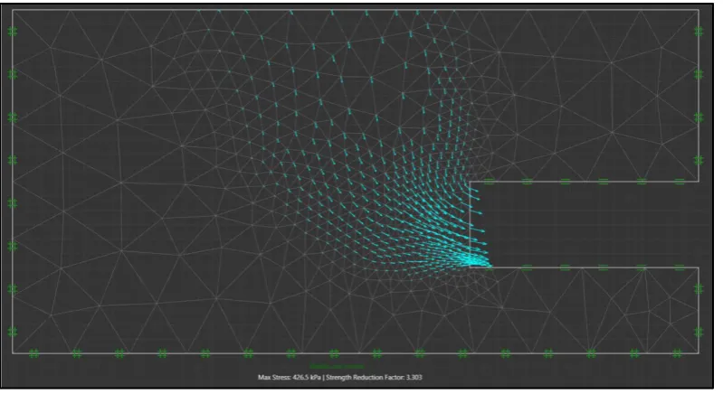
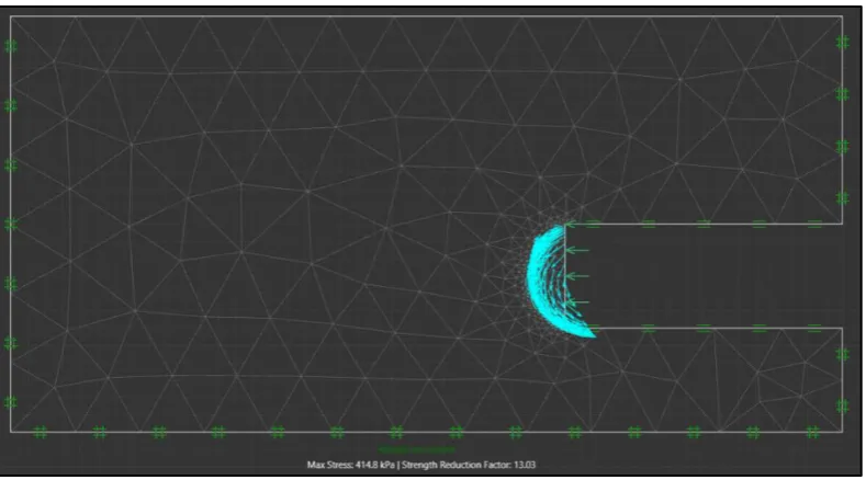
Figure 5.9: Tunnel heading failure by blowout showing displacement vector field. PR = -5, DR = 2 & SR = 1.50. ... 83

Figure 5.10: Plot of factor of safety verse pressure ratio for tunnel heading problem, DR = 2 and SR = 1.50. ... 84

Figure 5.15: Displacement vector field. PR = -2, DR = 2, SR = 1.50 ... 86

Figure 5.16: Factor of safety vs. strength ratio for all negative pressure ratios. DR = 1. 87 Figure 5.17: Factor of safety vs. strength ratio for all negative pressure ratios. DR = 2. 88 Figure 5.18: Factor of safety vs. strength ratio for all negative pressure ratios. DR = 3. 88 Figure 5.19: Factor of safety vs. strength ratio for DR = 2, PR = -3. ... 90

(13)

xii

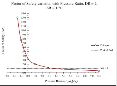
Figure 6.4: Displacement vector field for intermediate weightless scenario, DR = 2, SR =

1.50, PR = -1.75, corresponding FoS =13.09. ... 101

Figure 6.5: Factor of safety variation with pressure ratio for all strength ratios. DR = 2. ... 102

Figure 6.6: Tunnel heading stability design chart for DR = 1. ... 103

Figure 6.9: Tunnel heading stability design chart for SR = 0.10. ... 105

Figure 6.14: Tunnel Heading Stability Design Chart for SR = 1.10. ... 108

(14)

xiii

TABLE OF TABLES

(15)

1

CHAPTER 1:

INTRODUCTION

1.1

Outline of Study

This paper is focused on investigating tunnel heading stability for various cases of shallow tunnelling in undrained clay. A two-dimensional tunnel analysis was conducted for various scenarios where the load parameter, or pressure ratio as it will be referred to in this paper, was equal to zero, greater than zero and less than zero. Varying the pressure ratio allowed for the investigation of tunnel heading failure related to both the collapse and blowout mechanisms, with additional focus on the blowout failure mechanism due to the lack of previous research in this area. Ultimately, the factor of safety method was used to establish new safety design charts to assist engineers in the preliminary stages of tunnel design. Prior to this, a full understanding of tunnel heading stability must be obtained by reviewing and studying previous literature. Taylor (1937) applied the factor of safety approach to slope stability to develop Taylor’s slope stability design charts. The tunnel stability literature indicated that the stability of a tunnel is determined by predicting the limiting load that a tunnel can withstand prior to collapse. Broms and Bennermark (1967) were the first to develop this theory and apply it to tunnelling by deriving an initial stability number. By combining knowledge gained from Broms and Bennermark (1967) and Taylor (1937) it was possible to apply the factor of safety approach to tunnel heading stability.

(16)

2

the gravity is increased, or the strength is reduced, can be taken directly as the factor of safety. Results obtained from both methods were compared to each other and to external results obtained from a notable publication.

The failure mechanism of any scenario could be defined as either collapse, a downward soil movement, or blowout, an upward soil movement. The failure mechanism of each scenario was determined and discussed along with the relationship between the varying model input parameters. All results obtained from the Optum G2 analysis were presented in various stability design charts, which will possibly be useful to practicing engineers while in the preliminary stages of tunnel design. A number of select design examples were presented so the reader can better understand the application and usefulness of the design charts.

1.2

Methodology

The methodology for this research project was formulated in accordance with Appendix A – ‘Project Specification’ and is presented below in a number of basic steps.

1. Research literature relevant to tunnelling and in particular, tunnel heading stability. 2. Research literature related to the factor of safety approach and FELA.

3. Learn how to use Optum G2 by reading the manual and completing example problems.

4. Develop 2D models for shallow tunnel heading stability by varying the pressure ratio, depth ratio and strength ratio.

5. Perform an internal comparison of results obtained from the strength reduction and gravity multiplier methods, where applicable.

6. Compare Optum G2 shallow tunnel heading results with previously published results.

7. Discuss the failure mechanism for varying pressure ratios and the relationships between factor of safety, pressure ratio, strength ratio and depth ratio.

8. Develop stability design charts by applying the factor of safety approach.

9. Present and discuss a number of examples developed from the design stability charts.

(17)

3

1.3

Research Objectives

This study aimed to achieve a number of research objectives. The first, and broadest, objective was to gain a general knowledge of tunnel engineering with a focus on tunnel heading stability and to a lesser degree, tunnel construction methods. The ability to use Optum G2 to solve tunnel heading stability problems and apply the powerful new finite element limit analysis software to a broader spectrum of problems was another desired learning objective. It was also expected that a greater understanding of tunnel heading stability problems with a negative pressure ratio, having a failure mechanism similar to ‘uplift’ or ‘blowout’, will be obtained and transmitted through this paper, as it appears that this topic has not been thoroughly researched thus far. The research and modelling was expected to culminate in a new factor of safety approach, similar to slope stability, which can be applied to tunnel heading stability. The final output of this approach was a number of useful stability design charts for use by practicing engineers in the preliminary stages of tunnel design. An overview of the research objectives included; fully understand tunnel heading stability and its practical application, learn and utilise Optum G2, gain a higher level understanding of the blowout effect with regards to tunnel heading stability, develop a new theoretical factor of safety approach to tunnel heading stability and produce new design stability charts.

1.4

Organisation of Thesis

Chapter 2: General Review – This chapter introduces the concept and function of tunnels. A brief guide to tunnelling specific terminology is provided along with a summarised history of tunnelling, highlighting the most important breakthroughs throughout time. Modern tunnel construction techniques are discussed and the design criteria specific to tunnelling projects are outlined. A literature review of tunnel stability is conducted to assist in developing the factor of safety approach for tunnel stability.

(18)

4

Chapter 4: 2D Shallow Tunnel Heading Analysis: Collapse – This chapter introduces and defines the problem to be investigated, specifically, a shallow tunnel heading in undrained clay where the predominant failure mechanism can be related to collapse. The Optum G2 numerical modelling process is presented and the upper and lower bound factor of safety values are analysed and compared. The results obtained using the gravity multiplier and strength reduction methods are compared internally and then externally to previously published results. The relationship between the factor of safety and the defining dimensionless parameters, the pressure ratio, strength ratio and depth ratio will be investigated. The failure modes experienced are described by displaying the displacement vector fields. A final conclusion relating to shallow tunnel heading stability in undrained clay exhibiting a collapse failure mechanism is presented.

Chapter 5: 2D Shallow Tunnel Heading Analysis: Blowout – Similarly to chapter four, this chapter introduces and defines the problem to be investigated, specifically, a shallow tunnel heading in undrained clay where the predominant failure mechanism can be related to blowout. The significance of the blowout failure mechanism is highlighted and a historical example is provided. The Optum G2 numerical modelling process is presented and the upper and lower bound factor of safety values are analysed and compared. The results obtained using the gravity multiplier and strength reduction methods are compared internally to determine the most suitable method. The relationship between the factor of safety and the defining dimensionless parameters, the pressure ratio, strength ratio and depth ratio will be investigated. The failure modes experienced are described by displaying the displacement vector fields. A final conclusion relating to shallow tunnel heading stability in undrained clay exhibiting a blowout failure mechanism is presented.

(19)

5

heading stability in undrained clay and the development of stability design charts is presented.

(20)

6

2

CHAPTER 2:

GENERAL REVIEW

2.1

Introduction

In the world of civil engineering, tunnels are complex underground structures involving a number of challenging factors and unknowns not typically experienced when designing aboveground structures. No two tunnel construction projects will ever be identical, this is largely due to the complex and constantly varying nature of the soil medium. The soil medium is the body of soil through which the tunnel void passes. In tunnel construction the ground acts as both a loading and supporting mechanism, unlike other conventional structures which assume the soil provides a uniform foundation while timber, concrete and/or steel are provided as structural supports. Engineering judgement is especially important when designing and constructing tunnels as it is not possible to calculate discrete values for all surcharge loadings and soil properties and features that will be encountered while tunnelling. These factors are determined by soil testing and load calculations to a point, but are largely based on estimation and assumptions (Chapman, Metje & Stärk 2010). To develop the level of engineering judgement needed for tunnel design and construction an engineer must have a sound knowledge of construction processes, concrete engineering, structural analysis, mechanical engineering, hydraulic engineering and most importantly geology and geomechanics. An understanding of soil conditions, especially the strength and stability, and how they will affect the tunnelling process are of paramount importance.

2.2

Significance of Tunnels

(21)

7

2.3

Tunnelling Terminology

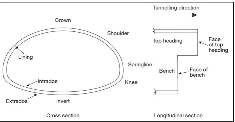
[image:21.595.101.499.247.455.2]

The method by which a tunnel is constructed depends on the purpose of the tunnel, site location, ground conditions, size, cost, and construction methods available. It is necessary to fully understand the different construction methods and the unique terminology relevant to each when designing a tunnel. However, to comprehend this research a basic understanding of key terminology is all that is required and any additional tunnel specific terms will be explained as they appear. Key tunnelling terminology is outlined below in Figure 2.1.

Figure 2.1: Terminology relevant to tunnel cross section and longitudinal section (Chapman, Metje & Stärk 2010).

2.4

History of Tunnels

(22)

8

Gunpowder was first used in tunnel construction in 1679 to build the tunnel that would become the pioneer of the Canal Age. The Canal du Midi was built between 1666 and 1681 and connected the Atlantic Ocean to the Mediterranean Sea. The 157 metre long tunnel section of the canal was necessary to pass under a ridge, and was the first tunnel on record that was constructed using gunpowder blasting as opposed to earlier fire setting techniques. The tunnel, which had a square cross section, was built between 1679 and 1681, and was originally unlined. In 1691 a structural lining was added to the tunnel.

It is well documented that Brunel’s great Thames Tunnel, a proposed dual carriageway under the Thames River in London, commencing in 1825, was the first shield driven tunnel and the first tunnel to pass under a tidal river. Sir Marc Isambard Brunel was the great mind behind Brunel’s Shield, the machine that revolutionised tunnelling and formed the primitive design basis of modern day tunnel boring machines. Brunel’s shield, shown in Figure 2.2, was designed to provide; a skin covering the ground on all sides, access for excavation while offering full face support and a means to move the shield forward into the excavated void while a brick lining was constructed behind it. The shield itself consisted of a cast iron framework, with twelve internal three tier frames. The earth in front of the shield was excavated with hand tools allowing the shield to be propelled forward by a number of screw jacks, which jacked off the completed brick lining. The tunnel was by far the most ambitious of its time and was eventually opened in 1842 as a pedestrian tunnel, after five inundations from the river above, many deaths and a great deal of over expenditure.

Figure 2.2: Brunel’s shield, a diagram showing a longitudinal section and one of the twelve frames (Guglielmetti et al. 2007).

(23)

9

problems were a big issue and this forced new developments in blasting and drilling techniques, such as compressed air rock drills. The first of these great Alpine tunnels to be constructed was the col de Frejus, a 12.23 kilometre long tunnel 1340 metres above sea level, carrying the railway from France to Turin. Mountain streams were used to provide ventilation and to compress air for the drills. Construction began in 1857 and was completed in 1871 by a workforce of approximately 4000 men.

1869 marked an important year for tunnelling development as it was the year that the subaqueous Tower subway in London was completed. The tunnel was constructed using a shield and cast iron lining and was used for a cable-hauled car, but now houses water mains. The 402 metre long tunnel was driven through clay nineteen metres below the water line and seven metres below the river bed. The shield mechanism used became known as Greathead’s shield and is known as the forefather of all modern day shields. It was during this project that grouting as a form of tunnel ground support was developed as well. The cast iron lining did not entirely fill the void so cement grout had to be injected to fill the gap between the lining and the soil. The Hudson River Tunnel, shown in Figure 2.3, was another important project of the time which also utilised Greathead’s shield and for the first time on a large scale tunnel, compressed air as a face stabilisation method. The soil/air pressure balance proved to be very unstable and after a serious accident, in which 20 lives were lost, the funding ran out and the tunnel was sealed off and left incomplete.

(24)

10

Maidl, Maidl and Thewes (2013) claimed that the first tunnel boring machine (TBM), where the entire machine face excavated the tunnel simultaneously using disc cutters, was constructed in 1851 and patented in 1856 by Charles Wilson. Wilson’s machine was trialled on the East portal of the Hoosac tunnel in Massachusetts. It soon became evident that the machine was not capable of tunnelling through the hard igneous rocks of New York. In 1875 Fredrick Beaumont obtained a patent to develop a new cutterhead design. Colonel English eventually took over this patent and by 1880 had developed a cutterhead which allowed for chisel heads to be exchanged without withdrawing the TBM. In the following years Beaumont successfully built two of England’s tunnel boring machines, shown below in Figure 2.4, and was involved in the partial construction of the Channel Tunnel. Over 1500 metres had been excavated either end of the tunnel before political reasons brought the project to a halt. The project was finally completed in 1994.

Figure 2.4: Illustration of English and Beaumont’s tunnel boring machine (Maidl, Maidl & Thewes 2013).

By the beginning of the 20th_{century many of the basic techniques involved in the}

construction of bored tunnels had been devised and proved through past success and failure. At this point in time tunnelling was considered a viable option so long as the developer was able to afford the process. This acceptance of tunnelling resulted in many new tunnel projects serving varied purposes throughout the world, including railways, metro systems, highway tunnels, water supply, sewer and waste removal, storage of goods and the housing of services such as pipes and cables. Tunnel boring machines underwent continual development and refinement throughout the 20th_{century. Throughout this time many}

(25)

11

across the world, improving the safety and efficiency of tunnel designs, Maidl, Maidl and Thewes (2013) further detail these modern advancements in tunnelling.

2.5

Tunnel Construction Methods

There are a number of different tunnel construction methods available to suit a range of different project conditions. Maidl, Maidl and Thewes (2013) have extensively researched and presented modern tunnel construction techniques. Presented in this section, will be a number of the most widely adopted methods used today.

The nature of the tunnel project will always be of paramount importance when determining the construction methods and techniques to be implemented. The function of the tunnel, location, soil conditions, nature of the obstacle being circumnavigated, tunnel dimensions, location of water table, tunnel depth, and quality of tests and available information all form part of the decision making process. Other factors affecting the project will include the timeline, finances, safety, noise, labour, available machinery and the environmental impact. There is no ‘one size fits all’ method available for tunnel construction and engineering judgement must be implemented to assess each project separately of all others.

Drill and blast tunnelling has been around in some form since the 17th_{century and has}

(26)

12

be in the form of timber, steel, grouting, anchors, dowelling or concrete. Artificial ventilation in the form of a ducting system is necessary when drilling and blasting to ensure that workers receive enough oxygen and the dust and fumes created from the blasting can be appropriately diluted.

Figure 2.5: Typical face drilling rig used in drill and blast tunnelling (Atlas Copco 2014).

(27)

13

when dealing with ground water pressure, it is common practice to use an earth pressure balance (EPB) machine or slurry shield machine. EPB machines were designed for use in cohesive soils and use the excavated soil to support the tunnel face. The excavated material is passed through a plenum where it is plasticised by mixing the soil with foams/slurry and other chemical additives before it is removed by a pressure controlled screw conveyor. The thrust force on the cutterhead, and the rate at which the material is removed through the screw conveyor, controls the pressure on the plenum. Slurry shield TBMs work on a similar principal to EPB machines but face support is provided by pressurising boring fluid (slurry) inside the cutterhead chamber. This boring fluid is generally a bentonite based slurry and is pumped to the cutterhead from a purpose built slurry plant. The slurry also acts as a means of removing the excavated soil as it is transferred back to the slurry plant where it is filtered and pumped back to the cutterhead for reuse through a system of pipes. Compressed air is sometimes used in conjunction with a slurry shield machine to help stabilise the face.

Figure 2.6: Diagram of typical tunnel boring machine with shield (Maidl, Maidl & Thewes 2013).

(28)

14

constructed within the trench, generally of cast in-situ concrete, precast concrete, corrugated steel arches or precast concrete arches. Once the tunnel is constructed, the trench is backfilled above the roof of the tunnel to restore the surface. Cut and cover tunnelling is limited to shallow constructions and a number of issues related to the construction’s short term and long term ability to resist water and lateral earth pressures can be encountered, especially when using ground anchors, diaphragm walls and sheet piling.

Figure 2.7: Example of bottom-up cut and cover tunnelling (Wallis 2002).

(29)

15

2.6

Design Criteria

Designing and building tunnels poses a great challenge to geotechnical engineers. The complexity and uncertainty of ground conditions along with the sensitive nature of the surface above are two of the biggest challenges incorporated in tunnelling. Guglielmetti, et al. (2007) outlined the primary design criteria to be considered when designing a tunnel as:

 The study of the settlement and consequent damage that the excavation could cause to the ground surface and existing structures above and around the tunnel, over both the short term and long term. This should include the consideration of any additional ground treatment or reinforcement that needs to be provided for existing structures.

 The design of the face support pressure for the excavation to ensure the required stability requirements are maintained throughout construction.

 The design of the tunnel’s final structural lining to ensure it can resist all earth and water pressure and current and future surcharge loading.

 The design of the tail void grouting to fill the space between the structural lining and the excavated earth void.

(30)

16

2.7

Tunnel Stability Review

As tunnelling technology developed and the transport needs of cities grew it became necessary, and possible, to build tunnels in increasingly challenging soil conditions. Many urban tunnels are constructed in saturated cohesive soils at shallow depths. A stability analysis must be performed as part of the initial tunnel design process to determine the feasibility of the project. The stability of tunnels has been researched through both two-dimensional and three-two-dimensional analysis. Two-two-dimensional tunnelling analyses have been extensively conducted for tunnel headings and tunnels with a circular or square cross section. Much of the research has focused on tunnels in an undrained cohesive soil medium. Undrained cohesive soil is a material where the internal angle of friction is equal to zero, this means that the undrained shear strength of the soil is simply equal to the cohesive strength of the soil. The stability of constructions in such soils can be quantified by a dimensionless stability number (N). The stability number was first proposed by Broms and Bennermark (1967) who performed extensive study on the plastic flow of clays at vertical faces. The stability number is defined in Equation 2.1.

𝑆𝑡𝑎𝑏𝑖𝑙𝑖𝑡𝑦 𝑁𝑢𝑚𝑏𝑒𝑟 (𝑁) =𝜎𝑠− 𝜎𝑡+ 𝛾(𝐶 + 𝐷 2) 𝑆𝑢

𝑤ℎ𝑒𝑟𝑒 𝜎𝑠= 𝑢𝑛𝑖𝑓𝑜𝑟𝑚 𝑠𝑢𝑟𝑐ℎ𝑎𝑟𝑔𝑒 𝑎𝑝𝑝𝑙𝑖𝑒𝑑 𝑎𝑡 𝑡ℎ𝑒 𝑠𝑢𝑟𝑓𝑎𝑐𝑒 [𝑁/𝑚2];

𝜎𝑡= 𝑖𝑛𝑡𝑒𝑟𝑛𝑎𝑙 𝑡𝑢𝑛𝑛𝑒𝑙 𝑝𝑟𝑒𝑠𝑠𝑢𝑟𝑒 [𝑁/𝑚2];

𝛾 = 𝑢𝑛𝑖𝑡 𝑤𝑒𝑖𝑔ℎ𝑡 𝑜𝑓 𝑡ℎ𝑒 𝑠𝑜𝑖𝑙 [𝑁/𝑚3_];

𝐶 = 𝑡𝑢𝑛𝑛𝑒𝑙 𝑐𝑜𝑣𝑒𝑟 [𝑚];

𝐷 = 𝑡𝑢𝑛𝑛𝑒𝑙 𝑑𝑖𝑎𝑚𝑒𝑡𝑒𝑟 [𝑚]; 𝑎𝑛𝑑

𝑆𝑢= 𝑢𝑛𝑑𝑟𝑎𝑖𝑛𝑒𝑑 𝑠ℎ𝑒𝑎𝑟 𝑠𝑡𝑟𝑒𝑛𝑔𝑡ℎ 𝑜𝑓 𝑡ℎ𝑒 𝑠𝑜𝑖𝑙 [𝑁/𝑚2].

Asadi and Sloan (1991) explain the theory of active and passive tunnel failure mechanisms. An active tunnel failure mechanism, or collapse, is created by the weight of the soil and surcharge pressure at the surface and is resisted by the internal tunnel pressure. A passive tunnel failure mechanism, or blowout, is created by the pressure in the tunnel and resisted by the weight of the soil and the surcharge pressure at the surface. A lot of previous work has been performed to develop and better understand the stability number and its application to slopes and tunnelling. Broms and Bennermark (1967) were the first to introduce the stability number as it is known today, and their work ventured into both the theoretical and practical application of the stability number and its application to a circular

(31)

17

void. Peck (1969) studied the theoretical stability number and further developed the design criteria for a circular section. Numerous experiments were conducted at the University of Cambridge during the 1970’s by Cairncross (1973), Seneviratine (1973) and Mair (1979) on the stability of circular tunnels in cohesive soil. The experiments involved modelling a tunnel and using a centrifuge to increase the gravity until a state of collapse was reached. This experimental method was again employed by Idinger, et al. (2011) who further investigated the stability of tunnel headings. Atkinson and Potts (1977) applied the upper and lower bound limit theorem to non-cohesive soils which was followed up by Davis, et al. (1980) who applied the upper and lower bound theorem to undrained cohesive soil. The upper and lower bound solutions provide a range for the factor of safety rather than an exact value, allowing the user to make a more informed decision on the factor of safety to be adopted. The pressure ratio of a homogeneous soil medium was established as a function of two independent parameters. Equation 2.2 shows the revised pressure ratio.

𝑃𝑟𝑒𝑠𝑠𝑢𝑟𝑒 𝑅𝑎𝑡𝑖𝑜 (𝑃𝑅) =𝜎𝑠− 𝜎𝑡 𝑆𝑢

= 𝑓 (𝐶 𝐷,

𝛾𝐷 𝑆𝑢

)

𝑤ℎ𝑒𝑟𝑒 𝐶

𝐷= 𝑡ℎ𝑒 𝑑𝑒𝑝𝑡ℎ 𝑟𝑎𝑡𝑖𝑜; 𝑎𝑛𝑑 𝛾𝐷

𝑆𝑢 = 𝑡ℎ𝑒 𝑠𝑡𝑟𝑒𝑛𝑔𝑡ℎ 𝑟𝑎𝑡𝑖𝑜.

Finite element limit analysis techniques are constantly improving, with researchers like Sloan (1988, 1989) and Lyamin and Sloan (2002a, 2002b) at the forefront of development. This constant advancement has meant that the method followed by Davis, et al. (1980) has been adopted to develop numerous tunnel stability research papers. These research projects modelled a range of geometrical tunnel profiles, including circular, square, rectangular, twin circular and tunnel heading, in a number of different soil mediums with varying material properties and complex loading conditions. The accuracy of results obtained from the lower and upper bound theorem were continually improving as the finite element limit analysis method was further researched. Sloan (2013) summarised the advancements of the finite element limit analysis method and describes how the upper and lower bound values are obtained by combining the finite element method with the limit theorems of classical plasticity.

Wilson, et al. (2011, 2013) investigated the stability of circular and square tunnel geometries through a two-dimensional plane strain analysis. It was assumed that the shear strength of the soil increased linearly with depth, meaning that another dimensionless

(32)

18

parameter was included in the stability problem. Equation 2.3 defines the stability number adopted for the square tunnel stability research.

𝑁 =𝜎𝑠− 𝜎𝑡 𝑐𝑢0

= 𝑓 (𝐻 𝐵,

𝛾𝐵 𝑐𝑢0

,𝜌𝐵 𝑐𝑢0

)

𝑤ℎ𝑒𝑟𝑒 𝑐𝑢0= 𝑢𝑛𝑑𝑟𝑎𝑖𝑛𝑒𝑑 𝑠ℎ𝑒𝑎𝑟 𝑠𝑡𝑟𝑒𝑛𝑔𝑡ℎ 𝑜𝑓 𝑠𝑜𝑖𝑙 𝑎𝑡 𝑠𝑢𝑟𝑓𝑎𝑐𝑒 [ 𝑁 𝑚2] ;

𝜌 = 𝑠𝑜𝑖𝑙 𝑠𝑡𝑟𝑒𝑛𝑔𝑡ℎ 𝑓𝑎𝑐𝑡𝑜𝑟;

𝐻 = 𝑑𝑒𝑝𝑡ℎ 𝑜𝑓 𝑡𝑢𝑛𝑛𝑒𝑙 [𝑚];

𝐵 = 𝑡ℎ𝑒 𝑡𝑢𝑛𝑛𝑒𝑙 𝑠𝑖𝑑𝑒 𝑙𝑒𝑛𝑔𝑡ℎ [𝑚]; 𝛾𝐷

𝑐𝑢0

= 𝑠𝑡𝑟𝑒𝑛𝑔𝑡ℎ 𝑟𝑎𝑡𝑖𝑜 𝑛𝑜𝑟𝑚𝑎𝑙𝑖𝑠𝑒𝑑 𝑡𝑜 𝑠𝑜𝑖𝑙 𝑠𝑡𝑟𝑒𝑛𝑔𝑡ℎ 𝑎𝑡 𝑠𝑢𝑟𝑓𝑎𝑐𝑒 ; 𝑎𝑛𝑑

𝜌𝐷 𝑐𝑢0

= 𝑠𝑡𝑟𝑒𝑛𝑔𝑡ℎ 𝑖𝑛𝑐𝑟𝑒𝑎𝑠𝑒 𝑛𝑜𝑟𝑚𝑎𝑙𝑖𝑠𝑒𝑑 𝑡𝑜 𝑠𝑢𝑟𝑓𝑎𝑐𝑒 𝑠𝑜𝑖𝑙 𝑠𝑡𝑟𝑒𝑛𝑔𝑡ℎ.

The strength factor (ρ) denotes the rate of strength increase with depth. The tunnel pressure, soil strength and soil strength factor must be normalised to the undrained shear strength of the soil at the surface (cu0) to account for the increase of soil strength with depth.

For both studies conducted by Wilson, et al. (2011, 2013) the strength increase ratio was varied from zero to one. It is important to note that when the strength increase ratio is equal to zero the soil medium is classified as homogeneous. The upper and lower bound results obtained through the finite element limit analysis were compared to results obtained by a more conventional semi-analytical rigid block analysis. It was found that the upper and lower bound results from the finite element limit analysis were in very good agreeance with the rigid block results. Figure 2.8 shows an example of the stability chart developed for an undrained square tunnel with H/B equal to two.

(33)

19

Figure 2.8: Design stability chart for square tunnel, H/B=2 (Wilson et al. 2013).

(34)

20

2.8

Factor of Safety Approach

Tschuchnigg, Schweiger and Sloan (2015) note that in the realm of geotechnical engineering there is no unique definition for the factor of safety. Bearing capacity problems usually define the factor of safety with respect to load capacity whereas slope stability problems usually define the factor of safety in relation to the soil strength. This research is based off the latter definition. The stability number can be further simplified by assuming an unsupported tunnel under Greenfield conditions and neglecting the surcharge pressure (σs) and the internal tunnel pressure (σt). In this scenario the pressure ratio is equal to zero.

Letting the pressure ratio equal zero reduces the problem to a familiar format seen when analysing the stability of a simple slope. Das (2010) describes the factor of safety in a homogeneous clay soil as the ratio of the soil’s undrained shear strength to the average shear stress developed along the potential failure plane. The factor of safety against sliding, shown in Equation 2.4, is developed by taking the moment of resistance.

𝐹𝑜𝑆 =𝑆𝑢 𝐶𝑑

𝑤ℎ𝑒𝑟𝑒 𝐹𝑜𝑆 = 𝑡ℎ𝑒 𝑓𝑎𝑐𝑡𝑜𝑟 𝑜𝑓 𝑠𝑎𝑓𝑒𝑡𝑦; 𝑎𝑛𝑑

𝐶𝑑= 𝑡ℎ𝑒 𝑐𝑜ℎ𝑒𝑠𝑖𝑜𝑛 𝑑𝑒𝑣𝑒𝑙𝑜𝑝𝑒𝑑 𝑡𝑜 𝑖𝑛𝑑𝑢𝑐𝑒 𝑓𝑎𝑖𝑙𝑢𝑟𝑒 [𝑁/𝑚2].

The minimum factor of safety value could relate to failure in the form of either a toe, midpoint or slope circle. Figure 2.9(a) shows a detailed diagram of a midpoint circle. The critical stability number for a slope circle is given in Equation 2.5.

𝑚 = 𝐶𝑑

𝛾𝐻= 𝑓 (𝛽, 𝐷 𝐻)

𝑤ℎ𝑒𝑟𝑒 𝑚 = 𝑠𝑙𝑜𝑝𝑒 𝑠𝑡𝑎𝑏𝑖𝑙𝑖𝑡𝑦 𝑛𝑢𝑚𝑏𝑒𝑟;

𝛽 = 𝑠𝑙𝑜𝑝𝑒 𝑎𝑛𝑔𝑙𝑒 [°];

𝐷 = 𝑑𝑒𝑝𝑡ℎ 𝑓𝑎𝑐𝑡𝑜𝑟 [𝑚]; 𝑎𝑛𝑑

𝐻 = ℎ𝑒𝑖𝑔ℎ𝑡 𝑜𝑓 𝑠𝑙𝑜𝑝𝑒 [𝑚].

The depth function using this method is defined as the ratio of the total depth, from the top of the slope to the solid base layer, to the height of the slope. The critical height which limits a slope to a minimum factor of safety can be found from Figure 2.9(b).

(2.4)

(35)

21

Figure 2.9: (a) Midpoint circle diagram outlining parameters; (b) Stability number plotted against slope angle (Das 2010).

Taylor (1937) developed a stability coefficient (Ns), defined in Equation 2.6 which relates to a critical failure surface where the factor of safety is a minimum.

𝑁𝑠=

𝑆𝑢

(𝐹𝑜𝑆)𝛾𝐻= 𝑓(𝛽, 𝐷)

𝑤ℎ𝑒𝑟𝑒 𝑆𝑢= 𝑢𝑛𝑑𝑟𝑎𝑖𝑛𝑒𝑑 𝑠ℎ𝑒𝑎𝑟 𝑠𝑡𝑟𝑒𝑛𝑔𝑡ℎ 𝑜𝑓 𝑠𝑜𝑖𝑙 [𝑁/𝑚2];

𝐹𝑜𝑆 = 𝑓𝑎𝑐𝑡𝑜𝑟 𝑜𝑓 𝑠𝑎𝑓𝑒𝑡𝑦; 𝑎𝑛𝑑

𝐷 = 𝑑𝑒𝑝𝑡ℎ 𝑓𝑎𝑐𝑡𝑜𝑟.

(36)

22

For a critical situation the factor of safety (FoS) is equal to one. This allows for the limiting dimensions of slopes to be calculated. The factor of safety for a slope problem can be rearranged, as in Equation 2.7, and shown as a function of the depth function, slope angle and strength ratio.

𝐹𝑜𝑆 = 𝑓(𝐷 𝐻, 𝛽,

𝑆𝑢

𝛾𝐻, )

A similar approach to that employed by Taylor can be applied to the stability of tunnels. The purpose of this study is to apply the factor of safety approach to tunnel heading stability problems with a non-zero pressure ratio. This study uses the finite element limit analysis technique to determine factor of safety values for a broad range of undrained tunnel heading stability problems. The factor of safety to be defined in this study is also a function of a number of dimensionless parameters similar to the factor of safety defined in Equation 2.7. The dimensionless parameters are varied within a practical range to ensure that results are applicable to a broad spectrum of real life scenarios. The factor of safety results will then be used to develop a number of stability design charts, similar to Taylor’s slope stability charts, but applicable to the preliminary stages of tunnel design.

(37)

23

3

CHAPTER 3:

NUMERICAL MODELLING REVIEW

3.1

Optum G2 Introduction

Optum G2 is a finite element limit analysis (FELA) software package designed for analysing the stability and deformation of a wide variety of geotechnical scenarios. Optum G2 is a relatively new program, it utilises a graphical user interface and shares many common features with other popular geotechnical analysis software. However, this software differs from conventional stability analysis software in the way that it is able to rigorously calculate upper and lower bound values for the factor of safety. This upper and lower bound theorem allows the user to calculate an average value for the factor of safety while also being aware of the worst case failure scenario. Another unique feature incorporated in the software is the ability to use automatic adaptive mesh refinement to maximize the accuracy of results. These features, coupled with the program’s user-friendly interface and powerful processing abilities make it suitable for analysing a broad range of two-dimensional plane strain geotechnical problems (Optum CE 2013).

Some may argue that since a tunnel is a three-dimensional structure it must be analysed in 3D. However, a 2D analysis has a number of benefits over a 3D analysis including; fast model setup and analysis times, low cost, a more user friendly and accessible process and a more conservative factor of safety than 3D modelling. In projects where the absolute highest accuracy is necessary and 2D modelling cannot supply a factor of safety that meets the design requirements then it is necessary to resort to 3D modelling.

3.2

Finite Element Limit Analysis

(38)

24

layered soil profiles, pore water pressures, anisotropic strength characteristics, staged construction and complex loadings in up to three dimensions.

Lysmer (1970) investigated the lower bound finite element limit analysis theorem and focused on optimizing the method’s application to plane strain soil mechanics problems. Pastor and Turgeman (1976) and Bottero, et al. (1980) investigated the upper bound limit analysis theorem and its application to two-dimensional plane strain problems involving Tresca and Mohr-Coulomb material. These early research projects focused on slope stability and the pulling out of foundations. Lyamin and Sloan (2002b) further explored the upper bound limit analysis theorem with the only unknowns being the plastic multiplier, nodal velocities and elemental stresses. Further research and significant optimization of the lower bound limit analysis theorem was performed by Lyamin and Sloan (2002a). Sloan (2013) analysed extensive literature related to the advancement of the finite element limit analysis theorem and its application to geotechnical stability analysis. A number of practical examples were presented covering; slopes, excavations, anchors, foundations and tunnels.

3.3

Gravity Multiplier Method

The gravity multiplier method (GMM) is an inbuilt method of analysis within the FE limit analysis software. Like its name suggests, it operates by increasing the gravity constant (g) gradually until a state of failure is reached. All other parameters remain the same and the factor by which the gravity is multiplied to cause failure is equivalent to the factor of safety. When using the gravity multiplier method the factor of safety can be defined as shown in Equation 3.1.

𝐹𝑎𝑐𝑡𝑜𝑟 𝑜𝑓 𝑆𝑎𝑓𝑒𝑡𝑦 (𝐹𝑜𝑆) =𝑔𝑐𝑟 𝑔

𝑤ℎ𝑒𝑟𝑒 𝑔𝑐𝑟 = 𝑡ℎ𝑒 𝑔𝑟𝑎𝑣𝑖𝑡𝑎𝑡𝑖𝑜𝑛𝑎𝑙 𝑎𝑐𝑐𝑒𝑙𝑎𝑟𝑎𝑡𝑖𝑜𝑛 𝑎𝑡 𝑓𝑎𝑖𝑙𝑢𝑟𝑒 [𝑚/𝑠2]; 𝑎𝑛𝑑

𝑔 = 𝑡ℎ𝑒 𝑎𝑐𝑡𝑢𝑎𝑙 𝑔𝑟𝑎𝑣𝑖𝑡𝑎𝑡𝑖𝑜𝑛𝑎𝑙 𝑎𝑐𝑐𝑒𝑙𝑎𝑟𝑎𝑡𝑖𝑜𝑛 = 9.81[𝑚/𝑠2].

The gravity multiplier method is not overly labour intensive on the computer’s processor, allowing for a fast and generally rather accurate solution when the pressure ratio equals zero. This method was used alongside, and compared to, the strength reduction method

(39)

25

when computing the factor of safety bounds for tunnel heading problems with varying pressure ratios.

3.4

Strength Reduction Method

The strength reduction method (SRM) is not dissimilar to the gravity multiplier method. When using the strength reduction method the strength properties of the soil are incrementally decreased until a limit of failure is reached. All other model and loading parameters remain the same and the factor by which the soil’s strength is reduced is equivalent to the factor of safety. When using the strength reduction method the factor of safety can be defined as shown in Equation 3.2.

𝐹𝑎𝑐𝑡𝑜𝑟 𝑜𝑓 𝑆𝑎𝑓𝑒𝑡𝑦 (𝐹𝑜𝑆) = 𝑆𝑢 𝑆𝑢.𝑐𝑟

𝑤ℎ𝑒𝑟𝑒 𝑆𝑢= 𝑜𝑟𝑖𝑔𝑖𝑛𝑎𝑙 𝑢𝑛𝑑𝑟𝑎𝑖𝑛𝑒𝑑 𝑠ℎ𝑒𝑎𝑟 𝑠𝑡𝑟𝑒𝑛𝑔𝑡ℎ 𝑜𝑓 𝑡ℎ𝑒 𝑠𝑜𝑖𝑙 [𝑁/𝑚2]; 𝑎𝑛𝑑

𝑆𝑢.𝑐𝑟= 𝑢𝑛𝑑𝑟𝑎𝑖𝑛𝑒𝑑 𝑠ℎ𝑒𝑎𝑟 𝑠𝑡𝑟𝑒𝑛𝑔𝑡ℎ 𝑜𝑓 𝑡ℎ𝑒 𝑠𝑜𝑖𝑙 𝑎𝑡 𝑓𝑎𝑖𝑙𝑢𝑟𝑒 [𝑁/𝑚2].

Many other finite element programs such as Plaxis and FLAC also utilise the strength reduction method. Tschuchnigg, Schweiger and Sloan (2015) described the strength reduction technique as a displacement-based finite element method and noted that a reasonable agreement is usually made between strength reduction methods and FELA methods for slope stability problems. When using Mohr-Coulomb soil properties the strength properties that are reduced are the cohesive strength and the internal angle of friction. If Tresca material properties are assumed, as they are in this study, the strength reduction process is simplified and only the cohesive strength of the soil is decreased, as the internal angle of friction is already equal to zero when dealing with undrained clay. The strength reduction method has seen extensive use in slope stability analysis and is growing in popularity and acceptance for tunnel stability analysis. Cai, Ugai and Hagiwara (2002) compared the finite element strength reduction method to the limit equilibrium method for circular excavations in soft clay and found the two to have a good degree of agreement. Huang, et al. (2012) again used the strength reduction method to investigate the stability of shallow tunnels in a saturated soil medium and validated their initial results by comparing to other published results. The strength reduction method will be used extensively in this study to investigate the factor of safety for shallow tunnel headings where the pressure ratio is less than, equal to and greater than zero.

(40)

26

3.5

Optum G2 Modelling

Optum G2 is a finite element limit analysis software program designed to solve geotechnical problems. The program contains a myriad of features for solving simple problems right through to complex multi-staged projects. Upon opening the program the user will be greeted with a screen similar to the one shown in Figure 3.1. The pop-up in the foreground contains the option to start a new project, load an existing one, access the user manual, watch a number of instructional videos or run a variety of preprogrammed examples. The design grid is in the background with the stage, properties, project and customisation manager to the right, with the taskbar containing the four functional tabs; geometry, materials, features and results, above.

Figure 3.1: Optum G2 opening screen (Optum Computational Engineering 2016).

(41)

27

Once the model geometry has been established, the materials can be chosen. The program comes with a broad range of pre-programmed materials but it is also possible to input a new material. There are eight different categories of materials available; solids, fluids, plates, connectors, geogrids, hinges, pile rows and nail rows. The solid category is used to represent materials such as soil, concrete and rock. A number of soil modelling options are available including Mohr-Coulomb (MC) and Tresca. MC materials assume linear elasticity and exhibit a yield function dependant on the cohesive strength (c)and angle of friction of the soil (ф). There is a wide variety of predefined Mohr Coulomb materials including; soft clay, firm clay, stiff clay, loose sand, medium sand and dense sand. Tresca materials are dependent only on undrained shear strength (Su). Once the desired material

type has been chosen, a number of properties related to that material can be manually varied in the ‘Properties’ bar that appears on the right hand side of the screen. For a Mohr-Coulomb material these variable properties include; drainage, stiffness, strength, flow rule, tension cut-off, compression cap, fissures, unit weight, initial conditions and hydraulic model. For a Tresca material these variable properties are limited to; stiffness, strength, tension cut-off, unit weight, initial conditions and hydraulic conductivity. A simple model with multiple soil layers is shown in Figure 3.3.

(42)

28

Figure 3.3: Model showing a number of different material layers (Optum Computational Engineering 2016).

The features tab allows the user to set; flow BC, consolidation BC, boundaries, fixed loads, multiplier loads, anchors and connectors, soil support, mesh size and the focus section. It is necessary to set boundary conditions to prevent the model from moving in the ‘x’ or ‘y’ directions. A ‘full’ support prevents the model from moving in all directions, while a ‘normal’ support only prevents movement in the parallel direction and a ‘tangential’ support only prevents movement in the perpendicular direction. A fixed load is applied to represent constant loads such as surcharge on the soil or permanent internal tunnel support. A multiplier load is applied with a unit load to allow the solver to amplify the load until a state of failure is reached, this feature can be used to find the limiting load on a soil structure. A water table or fixed pressure can be easily added at this stage along with any soil supports such as anchors, geogrids, piles and soil nails. Figure 3.4 shows the mesh of a model with boundary conditions and a distributed surcharge pressure applied.

(43)

29

The stage manager can be selected from the tabs towards the bottom right of the screen. It is here that the analysis is set up and a multi-staged project can be created. The drop-down box titled ‘analysis’ is used to select the type of analysis to be performed, options include; limit analysis, strength reduction, mesh, seepage, initial stress, elastic, elastoplastic, multiplier elastoplastic and consolidation. This research focuses on using only the limit analysis and strength reduction options. Selecting limit analysis allows the user to choose either a gravity or load multiplier, while selecting strength reduction allows the user to choose whether the strength of the solids or structures will be reduced. Both methods require that a time scope be chosen, either short or long term, to indicate whether the changes to the model will happen immediately or over a longer period of time. When analysing a problem in undrained clay it is necessary to use a long term analysis, but for sand, gravel or other coarse materials a short and long term analysis should be assigned to fully evaluate the problem. The element type can be set to upper, lower, six or fifteen element Gauss or a custom user specified element type. This study will focus on using only the lower and upper element types to ascertain the upper and lower bound factor of safety values. The number of elements in the initial mesh can be defined to influence the accuracy of the solution. Mesh adaptivity is a feature unique to Optum G2 and is used to perform adaptive mesh iterations to refine the failure mechanism and further increase the accuracy of results. For the gravity reduction and strength reduction methods it is recommended that at least three iterations be adopted along with shear dissipation as the adaptivity control (Optum CE 2013). The design approach can be set to provide a key factor of safety based on design codes but will be ignored and left as the default unity setting for this research. Figure 3.5 shows the stage manager.

(44)

30

Once the analysis has been performed through the stage manager window the outcome will be displayed in a pop-up screen and can be examined further through the results tab. A number of options are available to plot different features such as; displacement, strain, stress, material parameters, plastic multiplier, yield function and shear dissipation. An animation can be run to demonstrate the failure mechanism of the model. Results can be graphed, exported, generated in a report or viewed through a log. Figure 3.6 shows the results for a model that has been analysed using the lower bound gravity multiplier method, found under the limit analysis category. The animation of the model is shown at approximately eighty percent deformation scale with the mesh and plastic multiplier overlayed.

Figure 3.6: Solved model with deformation scale at eighty percent & plastic multiplier shown (Optum Computational Engineering 2016).

3.6

Optum G2 Slope Example

(45)

31

varying material layers will be analysed in this example to highlight the potential and simplicity of the software.

1. Create the geometrical model, defining any desired material layering.

Figure 3.7: Geometrical model of slope stability problem (Optum Computational Engineering 2016).

2. Define the restraints for the geometrical model so that the model as a whole is not able to move in the horizontal and vertical plane. Full restraints have been assigned to the base and sides of the model to prevent movement.

(46)

32

3. Select the materials required for each layer. In this case Soft MC, Firm Clay-MC and Stiff Clay-Clay-MC were chosen in the order of top to base layer.

Figure 3.9: Material types assigned to layers (Optum Computational Engineering 2016).

4. Apply loading conditions to the model. In this case a uniform surcharge of 10kPa will be applied.

(47)

33

5. Determine the type of analysis to be conducted and set up the stage manager accordingly. A lower and upper bound analysis using the strength reduction method (SRM) has been chosen in this example.

Figure 3.11: Stage Manager for upper and lower bound SRM (Optum Computational Engineering 2016).

6. Run analysis and view results log.

(48)

34

7. Analyse the results to determine a range of important information including; method of failure, max stresses, max shear and displacement.

Figure 3.13: Results of slope stability analysis showing fifty percent deformation and the plastic multiplier (Optum Computational Engineering 2016).

This basic example has illustrated how to perform a slope stability analysis on a simple slope with varying soil layers and a surcharge pressure in Optum G2. The process for analysing a tunnel problem is very similar and will be demonstrated in the following example.

3.7

Optum G2 Tunnel Heading Example

(49)

35

1. Create the geometrical model, defining any desired material layering. For this example a depth ration of two has been chosen, meaning the tunnel diameter is six metres and the cover above the tunnel is twelve metres. The model must be designed large enough so that boundary conditions do not adversely influence results.

Figure 3.14: Geometrical model for tunnel heading problem with depth ratio equals two (Optum Computational Engineering 2016).

2. Define the restraints for the geometrical model so that the model as a whole is not able to move in the horizontal and vertical plane. Full restraints have been assigned to the base and sides of the model while normal restraints are assigned to the roof and base of the tunnel excavation. The heading face has no restraints.

(50)

36

3. Assign materials to all layers of the model. This example assumes that the entire soil medium is homogeneous so will use only one material type. The chosen material is a Tresca Basic material with a specific weight of 18kN/m2_{and an}

undrained shear strength of 97.2kPa, resulting in a strength ratio of 0.9 when normalised to diameter.

Figure 3.16: Material type assigned to tunnel heading example (Optum Computational Engineering 2016).

4. Apply loading conditions to the model. In this case a surcharge pressure of 50kPa and an internal tunnel pressure of 50kPa will be applied, resulting in a pressure ratio equal to zero.

(51)

37

5. Determine the type of analysis to be conducted and set up the stage manager accordingly. A lower and upper bound analysis using the strength reduction method (SRM), followed by an upper and lower bound analysis using the gravity multiplier method has been established in this example.

Figure 3.18: Stage manager for upper and lower bound SRM and GMM (Optum Computational Engineering 2016).

6. Run analysis and view results log.

(52)

38

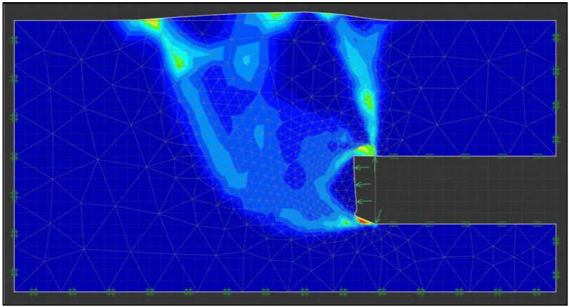
7. Analyse the results to determine a range of important information including; method of failure, displacement, max stresses and max strain.

Figure 3.20: Upper bound SRM results of tunnel heading example showing fifty percent deformation with mesh overlay (Optum Computational Engineering 2016).

(53)

39

Figure 3.22: Upper bound SRM results of tunnel heading example showing shear strain (Optum Computational Engineering 2016).

Figure 3.23: Upper bound SRM results of tunnel heading example showing σ1, σ2 vectors (Optum

(54)

40

Figure 3.24: Upper bound SRM results of tunnel heading example showing plastic multiplier (Optum Computational Engineering 2016).

(55)

41

4

CHAPTER 4:

TUNNEL HEADING ANALYSIS:

COLLAPSE

4.1

Introduction

As the world’s population grows and available space on the Earth’s surface decreases it is becoming increasingly necessary to construct subterranean infrastructure. As the need for tunnels increases so too does the required complexity of tunnelling projects. Tunnels present a unique challenge for engineers, who must assess the stability of prospective tunnels and the settlement of the Earth’s surface that could be caused by the tunnelling process. The safe design of tunnels is critical, especially in urban areas where a shallow void must pass under existing infrastructure sensitive to ground movement. Downward movement or collapse is the most common and easily understood tunnel failure mechanism. This chapter will address the tunnel heading stability problem for collapse by using Optum G2 to compute the upper and lower bound factor of safety values for a number of different scenarios. The relationship between the factor of safety and the three dimensionless parameters; depth ratio, strength ratio and pressure ratio, will be discussed with a focus on the collapse failure mechanism.

4.2

Problem Statement

In reality, tunnels are complex three-dimensional underground structures, however for the purpose of stability analysis they can be simplified to a basic two-dimensional model. The longitudinal section of the tunnel heading will be modelled under two-dimensional plane strain conditions. The undrained clay soil medium will be represented by a homogeneous Tresca material, which has an undrained shear strength (Su) and unit weight (γ). The cover

above the tunnel (C) and the height of the tunnel (D) are the important dimensional parameters needed to create the model. The surcharge pressure (σs) and internal tunnel

pressure (σt) are varied to test the stability of the model under a number of different pressure

(56)

42

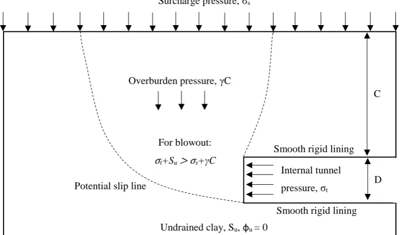
Figure 4.1 presents a conceptual model of the tunnel heading problem making it possible to comprehend the three important dimensionless variable parameters. The depth ratio (DR), shown in Equation 4.1, relates the geometrical properties of the model, tunnel height and tunnel cover. To represent shallow tunnelling conditions the depth ratio was varied between 1 and 3 in increments of one. Tunnel height remained constant at 6m while cover was varied.

𝐷𝑒𝑝𝑡ℎ 𝑅𝑎𝑡𝑖𝑜 (𝐷𝑅) =𝐶 𝐷

𝑤ℎ𝑒𝑟𝑒 𝐶 = 𝑐𝑜𝑣𝑒𝑟 𝑎𝑏𝑜𝑣𝑒 𝑡𝑢𝑛𝑛𝑒𝑙 [𝑚]; 𝑎𝑛𝑑 𝐷 = ℎ𝑒𝑖𝑔ℎ𝑡 𝑜𝑓 𝑡𝑢𝑛𝑛𝑒𝑙 𝑒𝑥𝑐𝑎𝑣𝑎𝑡𝑖𝑜𝑛 [𝑚].

The strength ratio (SR) can be represented in two different ways for this problem. The soil strength can be normalised to either the cover (C), as shown in Equation 4.2, or the tunnel height (D), as shown in Equation 4.3. Both formulations of the strength ratio were tested for this project and it was found that normalising the strength ratio to the tunnel height (D), as shown in Equation 4.3, produced the clearest and most effective results. To cover a broad range of practical scenarios the strength ratio (Su/γD) is varied between 0.10 and 2.00

in increments of 0.20 up to 1.50 and then a final increment of 0.50. Unit weight and tunnel height were kept constant at 18kN/m3_{and 6m respectively while undrained shear strength}

was varied.

Surcharge pressure, σs

Internal tunnel

pressure, σt Potential slip line

Smooth rigid lining

D C

Overburden pressure, γC

Undrained clay, Su, фu = 0

Figure 4.1: Tunnel heading stability problem statement. For collapse:

σs+γC > σt+Su

(57)

43

𝑆𝑡𝑟𝑒𝑛𝑔𝑡ℎ 𝑅𝑎𝑡𝑖𝑜 (𝑆𝑅) = 𝑆𝑢 𝛾𝐶

𝑆𝑡𝑟𝑒𝑛𝑔𝑡ℎ 𝑅𝑎𝑡𝑖𝑜 (𝑆𝑅) = 𝑆𝑢 𝛾𝐷

𝑤ℎ𝑒𝑟𝑒 𝑆𝑢= 𝑢𝑛𝑑𝑟𝑎𝑖𝑛𝑒𝑑 𝑠ℎ𝑒𝑎𝑟 𝑠𝑡𝑟𝑒𝑛𝑔𝑡ℎ 𝑜𝑓 𝑠𝑜𝑖𝑙 [𝑁/𝑚2]; 𝑎𝑛𝑑

𝛾 = 𝑢𝑛𝑖𝑡 𝑤𝑒𝑖𝑔ℎ𝑡 𝑜𝑓 𝑠𝑜𝑖𝑙 [𝑁/𝑚3].

The third dimensionless variable to be considered is the pressure ratio (PR). Classically this parameter has been defined as the load parameter but has been redefined as the pressure ratio in this project for simplicity and uniformity. The pressure ratio, shown in Equation 4.4, can be defined as the resultant applied pressure, be that a surcharge or internal tunnel pressure, compared to the undrained shear strength of the soil. To produce an acceptable range of data for modelling purposes the pressure ratio was varied between -16 and +10 with a focus on points ranging between -1.5 and +10 when analysing the collapse failure mechanism.

𝑃𝑟𝑒𝑠𝑠𝑢𝑟𝑒 𝑅𝑎𝑡𝑖𝑜 (𝑃𝑅) =𝜎𝑠− 𝜎𝑡 𝑆𝑢

𝑤ℎ𝑒𝑟𝑒 𝜎𝑠= 𝑡ℎ𝑒 𝑎𝑝𝑝𝑙𝑖𝑒𝑑 𝑠𝑢𝑟𝑐ℎ𝑎𝑟𝑔𝑒 𝑝𝑟𝑒𝑠𝑠𝑢𝑟𝑒 [𝑁/𝑚2]; 𝑎𝑛𝑑

𝜎𝑡= 𝑡ℎ𝑒 𝑎𝑝𝑝𝑙𝑖𝑒𝑑 𝑖𝑛𝑡𝑒𝑟𝑛𝑎𝑙 𝑡𝑢𝑛𝑛𝑒𝑙 𝑝𝑟𝑒𝑠𝑠𝑢𝑟𝑒 [𝑁/𝑚2].

The upper and lower bound factor of safety values are a function of these three dimensionless parameters and can therefore be expressed as shown in Equation 4.5.

𝐹𝑎𝑐𝑡𝑜𝑟 𝑜𝑓 𝑆𝑎𝑓𝑒𝑡𝑦 (𝐹𝑜𝑆) = 𝑓 (𝐶 𝐷,

𝑆𝑢

𝛾𝐷,

𝜎𝑠− 𝜎𝑡

𝑆𝑢

)

To gain a basic understanding of tunnel stability it is beneficial to first focus on a case where the pressure ratio is equal to zero. A pressure ratio of zero represents Greenfield conditions and means that the factor of safety is simplified to a function of only the depth ratio and strength ratio as shown in Equation 4.6.

𝐹𝑎𝑐𝑡𝑜𝑟 𝑜𝑓 𝑆𝑎𝑓𝑒𝑡𝑦 (𝐹𝑜𝑆) = 𝑓 (𝐶 𝐷,

𝑆𝑢

𝛾𝐷)

(4.2)

(4.3)

(4.4)

(4.5)

(58)

44

In previous tunnel heading stability literature the results and design charts are not expressed in a factor of safety format. They are generally represented as a stability number, which is a function of a particular depth ratio and strength ratio with a corresponding factor of safety of one. This stability number can generally cover a broader range of collapse failure scenarios when applied to a single design chart than a factor of safety approach, but is often confusing and somewhat impractical for practicing engineers