GOU, GANG. Efficient Algorithms for Querying Large-Scale Data in Relational, XML, and Graph-Structured Data Repositories. (Under the direction of Professor Rada Chirkova).
We live in an information age, and data are ubiquitous today. Various applications, ranging from scientific computing, medical research, and bioinformatics to administrative management, commercial sales, and financial marketing, generate and utilize data every day. Many of these applications are data intensive, with the amount of data involved potentially reaching hundreds of thousands of gigabytes. Further, different applications store data using different data models. For example, applications could store and manage structured data using a flat (relational) model, semi-structured data using a hierarchical (XML) model, and less-structured data using a more general and flexible graph model. In this thesis, I report my research results on efficiently querying large-scale data in relational, XML, and graph-structured data repositories.
XML, and Graph-Structured Data Repositories
by Gang Gou
A dissertation submitted to the Graduate Faculty of North Carolina State University
in partial fullfillment of the requirements for the Degree of
Doctor of Philosophy
Computer Science
Raleigh, North Carolina
2008
APPROVED BY:
Dr. Xiaohui Gu Dr. Ting Yu
Dr. Rada Chirkova Dr. Jon Doyle
DEDICATION
To my parents
Zhenghong Gou and Peixiu Wu
BIOGRAPHY
Gang Gou was born and grew up in Chongqing, a beautiful city in the west of China.
He studied in the Chongqing No. 29 Middle School from 1990 to 1996. He received the BSc degree in Computer Science from Nankai University, Tianjin, China, in June 2000, with the highest grade in his graduating batch. In August 2001 he moved to Hong Kong, China, and began to do research on database systems under the direction of Dr. Jeffrey Xu Yu, and then received the MPhil degree in Systems Engineering from the Chinese University of Hong Kong in July 2003. Since August 2003, he pursued his PhD studies under the direction of Dr. Rada Chirkova in Computer Science at North Carolina State University, Raleigh, NC, U.S.
His primary research interest is in database systems, with specialization in design-ing high-performance algorithms for efficient management and querydesign-ing of large-scale data arising in data-intensive applications. He has designed a number of high-performance algo-rithms for a variety of data-processing scenarios, with stored data ranging from structured data in traditional relational databases to the emerging semi-structured XML data and to the more complex graph-structured data in novel applications.
His research results have been published as full research papers in a number of lead-ing database conferences and journals, includlead-ing ACM SIGMOD (2006, 2007, and 2008)− the top conference in the area of database systems. He has also served as a referee for leading data management journals, including VLDB Journal, WWW Journal, and IEEE TKDE, and as an external reviewer for leading database conferences, including ACM SIG-MOD, ACM PODS, and VLDB. His research work has been supported by several federal-government-funded projects, including an U.S. NSF Career Award Project of Dr. Rada Chirkova.
ACKNOWLEDGMENTS
This dissertation would not have been completed without constant encourage-ments, supports, and help from many professors, friends, and my family.
First and foremost, I would like to acknowledge my Ph.D degree advisor, Dr. Rada Chirkova, for her insightful advice and continuous supports for my research work over the previous five years. Her wisdom and great guidance brought me lifelong skills that I will continue to benefit from in my future career. Also, I would like to thank my M.Phil degree advisor, Dr. Jeffrey Xu Yu, who brought me into the exciting database research area and taught me many preliminaries and fundamentals of doing database research. I am also grateful to Dr. Fereidoon Sadri, for his constructive discussions on database research in our weekly group reading meeting, and to Dr. Jun Yang, for his insightful comments and suggestions on earlier drafts of some of my publications. Also, I am grateful to my doctoral committee members, Dr. Jon Doyle, Dr. Xiaohui Gu, and Dr. Ting Yu, for their valuable suggestions on my research.
I would like to sincerely thank all members of our NCSU Database Group: Manik Chandrachud, Dongfeng Chen, Maxim Kormilitsin, and Zohreh Asgharzadeh Talebi, for their interesting discussions on research and on life and the happy times spent together in the office. I also thank Qunyi Chen, Xin Jin, and Xu Xu, the friends whom I met and knew in the NCSU Clark/Fountain dining hall. Chatting with them during lunch is always of happiness and fun. I also would like to thank all of other friends I met in Raleigh: David Johnson, Tiejun Li, Wei Tang, Wanhong Xu, Yipeng Yang, Qing Zhang, Yi Zhang, Jie Zhong, et al. Also, I am grateful to Heng Xia, my roomate who has lived with me in the same apartment for four years and witnessed most of my life in NCSU. In particular, I would like to thank Yifan Zhu, who helped me a lot when I was here in Raleigh. The weekly trip with him to the Grand Asia is always a nice experience in my life.
TABLE OF CONTENTS
LIST OF FIGURES . . . vii
1 Introduction . . . 1
1.1 Problems, Motivations, and Contributions . . . 2
1.1.1 Efficiently Querying Relational Databases . . . 2
1.1.2 Efficiently Querying XML Data . . . 5
1.1.3 Efficiently Querying Graph-Structured Data . . . 10
1.2 Organization of the Dissertation . . . 11
2 Efficient Algorithms for Querying Relational Databases . . . 12
2.1 Introduction . . . 12
2.1.1 Motivations . . . 14
2.1.2 Contributions . . . 17
2.2 Preliminaries . . . 19
2.2.1 Equivalent rewritings and views . . . 19
2.2.2 Our problem statement . . . 20
2.2.3 View tuples and efficient rewritings . . . 21
2.2.4 Query optimization under bag semantics . . . 23
2.3 Rewritings: Set Semantics . . . 24
2.3.1 Tuple coverages of view tuples . . . 24
2.3.2 Containment: partition condition . . . 25
2.3.3 Efficient algorithm for partition checking . . . 26
2.4 Cost-Based Query Optimizers for Bag-Set and Set Semantics . . . 32
2.4.1 Basic DP algorithm BDPV . . . 32
2.4.2 Complete algorithm CDPV . . . 34
2.5 Related Work . . . 35
2.6 Conclusion . . . 36
3 Efficient Algorithms for Querying XML Data . . . 38
3.1 Introduction . . . 38
3.1.1 Preliminaries . . . 38
3.1.2 Related Work . . . 41
3.1.3 Motivations and Contributions . . . 43
3.2 Lazy Filtering Algorithm (LF) . . . 44
3.2.1 Query Preprocessing . . . 44
3.2.2 The Basic LF Algorithm (B-LF) . . . 46
3.2.3 The Full LF Algorithm (LF) . . . 49
3.3 Lazy Querying Algorithm (LQ) . . . 51
3.3.1 Query Preprocessing . . . 51
3.3.3 The Full LQ Algorithm (LQ) . . . 55
3.4 Eager Querying Algorithm (EQ) . . . 57
3.4.1 Query Preprocessing . . . 57
3.4.2 Algorithm . . . 58
3.5 Experimental Results . . . 64
3.5.1 Experimental Setup . . . 64
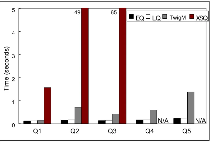
3.5.2 Time Performance . . . 65
3.5.3 Memory Space Performance . . . 69
3.5.4 Summary . . . 72
3.6 Conclusion . . . 72
4 Efficient Algorithms for Querying Graph-Structured Data . . . 74
4.1 Introduction . . . 74
4.1.1 Motivations . . . 75
4.1.2 Problem Definition . . . 76
4.1.3 Contributions . . . 77
4.2 Run-Time Graph . . . 77
4.3 The Architecture . . . 79
4.4 Our Algorithm DP-B . . . 81
4.4.1 FQ-iterator . . . 82
4.4.2 FR-iterator . . . 89
4.4.3 The DP-B Algorithm . . . 92
4.5 Our Algorithm DP-P . . . 95
4.6 Related Work . . . 104
4.7 Experiments . . . 106
4.8 Conclusion . . . 112
5 Conclusion . . . 113
5.1 Summary of Contributions . . . 113
5.2 Future Work . . . 115
6 Proofs . . . 118
6.1 Preliminaries of the Proof for Theorem 5 in Section 2.3.2 . . . 118
6.2 Proof for Theorem 5 in Section 2.3.2 . . . 120
6.2.1 Tuple Coverage Partition ⇒ Containment Mapping . . . 120
6.2.2 Containment Mapping⇒ Tuple Coverage Partition . . . 122
6.3 Proof for Lemma 4 in Section 2.3.3 . . . 125
6.4 Proof for Theorem 13 in Section 4.4.3 . . . 126
LIST OF FIGURES
Figure 1.1 Answering queries using views: an example. . . 3
Figure 1.2 Examples of XML documents. . . 5
Figure 1.3 The XML data model. . . 7
Figure 1.4 Examples: XPath. . . 8
Figure 2.1 Query semantics. . . 13
Figure 2.2 The equivalence of the rewritings to the query: an example. . . 14
Figure 2.3 The equivalence of the rewritings to the query: data instances (1). . . 15
Figure 2.4 The equivalence of the rewritings to the query: data instances (2). . . 16
Figure 2.5 The search space of a view-based query optimizer (w.r.t. Figure 2.2). . . 17
Figure 3.1 Grammar of Univariate XPath. . . 39
Figure 3.2 Sub-patterns of an XPath queryQ. . . 40
Figure 3.3 Query table for the query of Figure 3.2. . . 45
Figure 3.4 B-LF (query: ‘//A[//D]//B[/E]/C’). . . 48
Figure 3.5 Mapping table (LF):name→ column sequence. . . 50
Figure 3.6 LF: Incorrect order of calling blocks (query: ‘//*[//A]/B/C’). . . 50
Figure 3.7 U-LQ (query: ‘//A[//D]/B[/E]//C’). . . 54
Figure 3.8 LQ (the same query/data as in Figure 3.7). . . 56
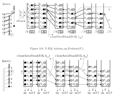
Figure 3.9 U-EQ: bottom up Evaluate(U). . . 61
Figure 3.10 U-EQ: top down Propagate(b10b14). . . 61
Figure 3.11 U-EQ (the same query/data as in Figure 3.7). . . 62
Figure 3.13 Queries for the experimental evaluation. . . 65
Figure 3.14 Query time for the Book dataset.6. . . 66
Figure 3.15 Query time for the Treebank dataset.6. . . 67
Figure 3.16 Query time for the XMark dataset.6. . . 68
Figure 3.17 Size of buffering space (number of nodes) for the Book dataset.6. . . 69
Figure 3.18 Size of buffering space (number of nodes) for the Treebank dataset.6. . . 70
Figure 3.19 Size of buffering space (number of nodes) for the XMark dataset.6. . . 71
Figure 4.1 Twig query and its run-time graph. . . 79
Figure 4.2 Nested iterators: the architecture.. . . 80
Figure 4.3 An fQ-k lattice (fQ= 3 and k= 3).. . . 82
Figure 4.4 (Example)aj.FQ: findingk closest descendants of root in anfQ-klattice for fQ= 3 and k= 5.. . . 86
Figure 4.5 0 or 1 fresh read. . . 88
Figure 4.6 FQ/FR-iterators of DP-B: time and space costs. . . 89
Figure 4.7 (Example) ai.FRC: performing fR-way merge for fR= 5 and k= 4. . . 91
Figure 4.8 DP-B and DP-P: time and space costs . . . 94
Figure 4.9 Running DP-B forQand GR in Figure 4.1 (k=2), with all iterators omitted. 96 Figure 4.10 Running DP-P forQandGRin Figure 4.1 (k=2), with all iterators omitted. 97 Figure 4.11 Query time (t) for Q1 over the Boost dataset.. . . 108
Figure 4.12 Query time (t) for Q2 over the Boost dataset.. . . 108
Figure 4.13 Query time (t) for Q3 over the Boost dataset.. . . 109
Figure 4.14 Query time (t) for Q4 over the DBLP dataset. . . 109
Figure 4.15 Query time (t) for Q5 over the DBLP dataset. . . 110
Figure 4.16 Query time (t) for Q6 over the DBLP dataset. . . 110
Figure 4.18 Query time interval (∆t) for Q4 over the DBLP dataset. . . 111
Chapter 1
Introduction
We live in an information age, and data are ubiquitous today. Various applications, ranging from scientific computing, medical research, and bioinformatics to administrative management, commercial sales, and financial marketing, generate and utilize data every day. Many of these applications are data intensive, with the amount of data involved potentially reaching hundreds of thousands of gigabytes. Whether these applications can efficiently manage and query such a large amount of data is no doubt one of the most important factors that determine their success or failure. Further, different applications could prefer different data models due to different application-specific characteristics of data. For example, applications could store and manage structured data using a flat (relational) model, semi-structured data using a hierarchical (XML) model, and less-structured data using a more general and flexible graph model.
In this thesis, I report my research results [1, 2, 3, 4] on efficiently querying large-scale data in different models, which range from structured data stored in traditional rela-tional databases (Chapter 2)1 to the emerging semi-structured XML data (Chapter 3)2 and
to the more complex graph-structured data arising in various applications (Chapter 4)3.
1An earlier version of this work [1] has been invited to present in the 35th ACM SIGMOD International Conference on Management of Data, Chicago, U.S., 2006.
2An earlier version of this work [2] has been invited to present in the 36th ACM SIGMOD International Conference on Management of Data, Beijing, China, 2007.
1.1
Problems, Motivations, and Contributions
1.1.1 Efficiently Querying Relational Databases
Many of today’s commercial database systems are relational database systems; examples include IBM DB2, Microsoft SQL Server, and Oracle DB. In my M.Phil research and earlier PhD research, I put a lot of effort into improving the query-processing per-formance of relational databases. Specifically, I explored the view-based approach, which precomputes and stores, or materializes, the results of ‘hot’ queries (i.e., those queries of significant interest to a large number of database users) as materialized views, with the motivation that many incoming queries could be answered directly using these (concise) precomputed views, instead of costly drilling down into the original very large data bases.
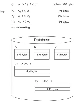
Example 1 Figure 1.1 gives a motivation example, in which the database includes three base relations A, B, and C, and two precomputed views V1 and V2. For each base rela-tion/view, we also identify its disk size in Figure 1.1.
On one hand, if there are no precomputed views, the queryQhas to be answered by joining three base relations, which incurs at least 16Mbytes disk I/O cost. (As traditionally, here we estimate the disk I/O cost of answering a query using the sum of the size of all input relations/views (as well as intermediate join results) of this query.)
On the other hand, with precomputed views, the cost of processing the queryQcan be reduced significantly. For example, the rewritingR3 of the query, which joins V1 andV2, incurs only 6Mbytes disk I/O cost. In this case, we call R3 the optimal rewriting of the queryQ, since it has the lowest cost among all rewritings of Q.
(Note that in this example we are temporarily taking the assumption that views have relatively smaller sizes than those of base relations. This is not always true in practice. However, the view-based query optimizers we propose in Chapter 2 work in a cost-based way. They automatically estimate and compare the cost of different rewritings of the query based on the sizes of bases relations and views (as well as intermediate join results) of these rewritings. As a result, the search space of our view-based query optimizers include both rewritings involving views and rewritings not involving views.)
Query: Q: A B C
Rewritings: R1: V1 C
V1: A B A
8 M bytes
B C
V2: B C
Database
R2: A V2
R3: V1 V2
Disk I/O Cost
at least 16M bytes
7M bytes
10M bytes
6M bytes
optimal rewriting
5 M bytes 3 M bytes
4 M bytes
2 M bytes
Answering Queries Using Materialized Views
In [1] we address the problem of answering queries using views. This problem is, given a user’s query Q and a set of precomputed views V, find an optimal (equivalent) rewritingR (say R3 in Example 1) ofQ that is composed of views in V.
We propose two novel view-based query-optimization algorithms to address this problem, and make the following contributions. (1) Our algorithms work under both bag-set and set query semantics that have been widely used in today’s relational databases. Under these semantics, the base relations (i.e., data tables) do not contain duplicate tuples, while the query results may or may not contain duplicate tuples. (2) Our algorithms work for a large and practically important subset of SQL queries, which includes not only conjunctive (Select-Project-Join) queries but also aggregate (SUM/COUNT/MAX/MIN) queries. (3) Our algorithms explore multiple-view rewritings as well as single-view rewritings of the query to guarantee the optimality of the rewritings they produce. (4) Our algorithms do cost-based System-R-style dynamic programming, and can be integrated easily into existing commercial relational query optimizers that do not use views. (5) In particular, we have done a theoretical and practical study of the completeness-efficiency trade-off between our two algorithms BDPV and CDPV. Our results show that BDPV could be preferable in practice, since it generally has much higher efficiency than CDPV (which provides higher-quality rewritings), while still finding high-higher-quality near-optimal rewritings.
In Chapter 2 I give a detailed introduction to our view-based query-optimization algorithms.
Materialized View Selection
It is usually impractical to materialize the results of all ‘hot’ queries, due to the system resource constraints − each materialized view incurs some disk-space costs and maintenance-time costs. For example, for the example in Figure 1.1, the views V1 and V2
incur 4Mbytes and 2Mbytes disk-space costs, respectively.
This motivates us to address the view-selection problem. That is, given a query workload WQ collected from the run-time statistics and a system resource constraint RC,
select an optimal set of views V to precompute, which maximize the total processing per-formance of all queries in WQ and meanwhile use no more than RC resources. Actually,
!" #$ ! ! % & & ! !" #$ ' ( ) * + ,-. '( ) * + ,-.
Figure 1.2: Examples of XML documents.
hard. Therefore, we focus on efficiently finding a near-optimal set of views. Specifically, we have proposed various algorithms, including anA∗ algorithm [5, 6, 7] and an evolutionary algorithm [8], to address this problem. Our algorithms can find high-quality view sets ef-ficiently in practice. In [9, 10] we also did an empirical study and comparison of existing greedy/heuristic view-selection algorithms. The above results have been reported in my Master’s thesis [7].
1.1.2 Efficiently Querying XML Data
Extensible Markup Language (XML) is emerging as a de facto standard for in-formation exchange among various applications on the World-Wide Web, due to XML’s inherent data self-describing capability and flexibility of organizing data [11]. There has been a growing need for developing high-performance techniques to query large XML data repositories efficiently.
an example of an XML document, which records information about publishers. However, unlike HTML, in which tags associated with data express the presentation style (e.g., font style) of data, tags in XML are intended to describe the semantics of data. For example, Lines 1-3 in Figure 1.2 (a) say that ‘Cambridge’ is an address of a publisher whose name is ‘M IT P ress’. This self-describing capability of XML data helps applications on the Web “understand” the content of XML documents published by other applications.
Second, XML is flexible in organizing data. The hierarchy formed by nested tags structurizes the content of XML documents. The role of nested tags in XML is somewhat similar to that of schemas in relational databases. At the same time, the nested XML model is far more flexible than the flat relational model. In an XML document, objects of the same type might have different types of sub-objects or different numbers of sub-objects of the same type. For example, in Figure 1.2 (a) the first publisher — but not the second
publisher — has anaddresssub-element. The bookunder the firstpublisher has two author
sub-elements, but the bookunder the second publisherhas only one.
XML Data Model
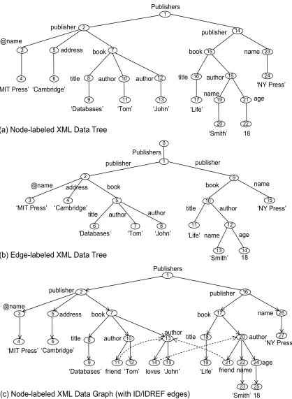
The basic data model of XML is a labeled and ordered tree. Figures 1.3 (a) and (b) show the data tree of the XML document of Figure 1.2 (a). Figure 1.3 (a) is based on thenode-labeledmodel, with labels on nodes, and Figure 1.3 (b) is based on theedge-labeled
model, with labels on edges. These two models are equivalent. We discuss XML data trees based on the node-labeled model; analogous points hold for the edge-labeled model. There are basically three types of nodes in a data tree: (1)Elementnodes (internal nodes), which correspond to tags in XML documents, e.g.,publisher. (2) Attributenodes (internal nodes), which correspond to attributes associated with tags in XML documents, e.g., ‘@name’. In contrast to element nodes, attribute nodes are not nested (i.e., an attribute cannot have any sub-elements), are not repeatable (i.e., two same-name attributes cannot occur under one element), and are unordered (i.e., attributes of an element can freely interchange their occurrence locations under the element). (3) Value nodes (leaf nodes), which correspond to data values in XML documents, e.g., ‘M IT P ress’. Edges in a data tree represent structural relationships between elements, attributes, and values.
(a) Node-labeled XML Data Tree
publisher publisher
address book book name
‘MIT Press’ ‘Cambridge’
title author author title author
‘Databases’ ‘Tom’ ‘Life’ age
‘Smith’ name ‘John’
18
‘NY Press’
(b) Edge-labeled XML Data Tree @name Publishers 10 11 12 13 14 15
(c) Node-labeled XML Data Graph (with ID/IDREF edges) 1
3
2
5 4
6 7 8
9
Publishers
publisher publisher
@name
address book book name
‘MIT Press’ ‘Cambridge’
title author author title author
‘Databases’ ‘Tom’ age ‘Life’ ‘Smith’ name ‘John’ 18 ‘NY Press’
friend loves friend
0 Publishers
publisher
publisher @name
address book book name
‘MIT Press’ ‘Cambridge’
title author author title author
‘Databases’ ‘Tom’ age ‘Life’ ‘Smith’ name ‘John’ 18 ‘NY Press’ 1 2 3 4 5 6 7 8 9 10 11 12 13 14 15 16 17 18 19 20 21 22 23 24 1 2 3 4 5 6 7 8 9 10 11 12 13 14 15 16 17 18 19 20 21 22 23 24 25 26 27
publisher
@name
book
title =‘MIT Press’
? publisher
title ?
(1) Path Pattern (2) Twig Pattern
Figure 1.4: Examples: XPath.
[12], multiple section nodes might be nested on the same path. Recursion occurs fairly frequently in XML data in practice. Choi et al. [13] investigated 60 DTDs, among which 35 are recursive. (DTD is a kind of schema of XML data [14].) As we shall see in Chapter 3, recursion in XML data significantly increases the complexity of efficiently querying XML data.
XML Queries
Unlike (flat) text documents, XML documents have nested structure. Thus, XML queries concern not only the content but also the structure of XML data. Basically, the queries can be formed using twig patterns, in which nodes represent the terms the user is interested in, i.e., the content part of queries, and edges represent the structural relationships the user wants to hold between the terms, i.e., the structural part of queries.
XPath [15] is a basic XML query language that selects nodes from XML documents, such that the path from the root to each selected node satisfies a specified pattern. A simple XPath query is formulated as a sequence of alternating axes and tags. Two most commonly used axes are the child axis, ‘/’, where ‘A/B’ denotes selecting B-tagged child nodes of A-tagged nodes, and the descendant axis, ‘//’, where ‘A//B’ denotes selecting B-tagged descendant nodes of A-tagged nodes. Consider an example: An XPath query ‘/publisher//title’ would return all title elements under all top-level publisher elements. The result of this query on the data tree of Figure 1.3 (a) is twotitlenodes that have values ‘Databases’ and ‘Life’, respectively.
represents the ‘//’ axis, and the shaded node is anoutput node. Generally, an XPath query can specify a more complex twig patternby usingpredicatesin its expression. One example is ‘/publisher[@name = ‘M IT P ress′]/book/title’, in which ‘/publisher/book/title’ is the main path of the query, and the content between ‘[’ and ‘]’ is a predicate on thepublisher. See also the twig pattern of this query in Figure 1.4 (2). This query returns all book titles of the publisher with name ‘M IT P ress’. Generally, an XPath query might involve nested predicates on multiple nodes in its twig pattern.
From the above we can see that the core of an XPath query is a twig pattern that includes exactly one output node. Further, we call nodes in query twig patternsquery nodes, and nodes in data trees data nodes.
Contributions
Due to the growing importance of XML in information exchange among various applications on the Web, many of today’s commercial database vendors are extending their database systems to support XML. Meanwhile, a large amount of research work has been done on efficiently managing and querying XML data. In [4] I did a review, analysis, and comparison of the state-of-the-art XML-querying techniques (from more than 120 publica-tions), including both relational techniques and native techniques.
Specifically, in my study of XML query processing, I focus on exploring a funda-mental problem of evaluating XPath queries over XML streams, motivated by a growing practical need for efficiently querying streaming XML data. In many emerging applications, such as monitoring stock market data, subscribing to real-time news, and managing network traffic information, XML data are available in streamingform only. An essential difference between querying streaming XML data and querying non-streaming XML data is that the former requires one-pass algorithms over unindexed XML data, in which all data have to be read sequentially and only once into memory.
algorithms that achieve the O(|D||Q|) time performance. (Building these algorithms also gives us an important result that XPath queries can be efficiently evaluated in the same O(|D||Q|) time in the streaming environment as in the non-streaming environment.) In particular, our algorithm EQ also achieves optimal space performance, which has not been achieved by any previous algorithms. Our extensive experimental results show that our algorithms are not only of high theoretical value but also have considerable practical time and space performance advantages over the state-of-the-art algorithms.
In Chapter 3 I give a detailed introduction to our XPath stream-querying algo-rithms LQ and EQ.
1.1.3 Efficiently Querying Graph-Structured Data Graph Data Model
Graph-structured data are ubiquitous today, and have been widely generated and used in many application domains, including bioinformatics, chemistry, networking, and semantic web. Essentially, in the object-oriented viewpoint, many types of data, including relational data and XML data, can be modeled as graph data, in which nodes represent objects, and edges represent relationships between objects.
A direct example of graph-structured data is from XML. In Section 1.1.2 we have seen that the basic data model of XML is a tree. Further, the tree model of XML can be extended to a graph model when ID/IDREF attributes are associated with elements in XML documents, where an ID attribute uniquely identifies an element in XML documents and
IDREF attributesrefer to other elements that are explicitly identified by their ID attributes. Figure 1.2 (b) shows an XML document with ID/IDREF attributes. ID/IDREF attributes increase the flexibility of the XML data model and extend the basic tree model to directed acyclic graphs (DAGs) or to even more general directed graphs with cycles. Figure 1.3 (c) shows an XML data graph with cycles, which corresponds to the XML document of Figure 1.2 (b).
Contributions
problem of answering twig queries over graphs, that is, finding the matches of a given twig-pattern query in graphs. We observe that a twig query could have an extremely large, potentially exponential, number of answer matches in a graph. Retrieving and returning to the user this many answers may both incur high computational overhead and overwhelm the user. Motivated by this, in [3] I propose two efficient algorithms, DP-B and DP-P, for retrieving top-ranked, specifically top-k, tree-pattern matches from large graphs, where k is a user-specified constant.
Our contributions are as follows. (1) Both DP-B and DP-P retrieve exact top-k answer matches from the space of potentially exponentially many matches in polynomial
time and space in the worst case. To the best of our knowledge, our algorithms are the first to have these excellent efficiency properties. (2) DP-B finds the first answer in time and space linear in the data size, while finding each of the followingk−1 answers incrementally in time and space that do not depend on the data size. That is, DP-B finds all exact top-k answers in time and space linear in the data size. (3) Further, we go beyond the linear-cost result of DP-B, and propose a more efficient algorithm DP-P. With powerful pruning techniques, DP-P could take far less than linear time and space cost in practice. (4) Our experimental results corroborate the high performance of both our algorithms in practice.
In Chapter 4 I give a detailed introduction to our efficient algorithms DP-B and DP-P.
1.2
Organization of the Dissertation
Chapter 2
Efficient Algorithms for Querying
Relational Databases
2.1
Introduction
We study the problem of finding efficient equivalent rewritings of relational queries using views. The problem has received significant attention because of its applications in a number of data-management problems [16], such as query optimization [17, 18, 19], maintenance of physical data independence [20, 21], and data warehousing [22, 23]. Our work focuses in particular on query optimization in presence of materialized views. Given a user query, the task of an optimizer is to search the space of all physical query plans for an optimal plan. Besides being correct, the process should be efficient, cost based, and as complete as possible. Traditional query optimizers such as the System-R optimizer [24] search in the space of left-deep join trees of a logical plan for an optimal physical plan, which specifies execution details such as join ordering and implementation of a join (e.g., hash join or sort-merge join).
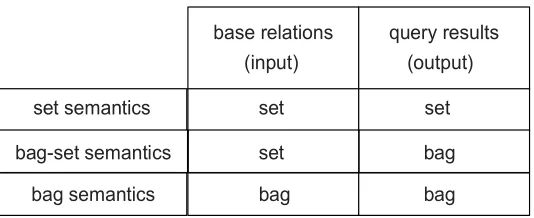
(input) set semantics
bag-set semantics bag semantics
set set bag base relations
(output) query results
bag bag set
Figure 2.1: Query semantics.
(i.e., is complete) for SPJ queries and views without inequality comparisons, under the assumption that both base relations and query answers can have multiple identical tuples — that is, under bag semanticsfor query evaluation [25].
We continue the line of work of [17] by studying query optimization using views in a System-R-style optimizer [24], for SPJ queries and views that may involve grouping and aggregation. We make an important assumption that base relations cannot contain duplicate tuples. In this setting there may exist efficient equivalent rewritings of a given query using given views such that these rewritings cannot be obtained using the approach of [17]. We distinguish between two possible scenarios:
• bag-set semantics for query evaluation [25], where duplicate tuples are retained in query answers, and
• set semantics, where duplicate tuples are eliminated from query answers.
Note that evaluation under bag-set semantics is essential for aggregate SQL queries involving aggregation functions SUM orCOUNT [26, 27], whereas, for instance, queries with the DISTINCT keyword must be evaluated under set semantics. Figure 2.1 compares bag, bag-set, and set semantics.
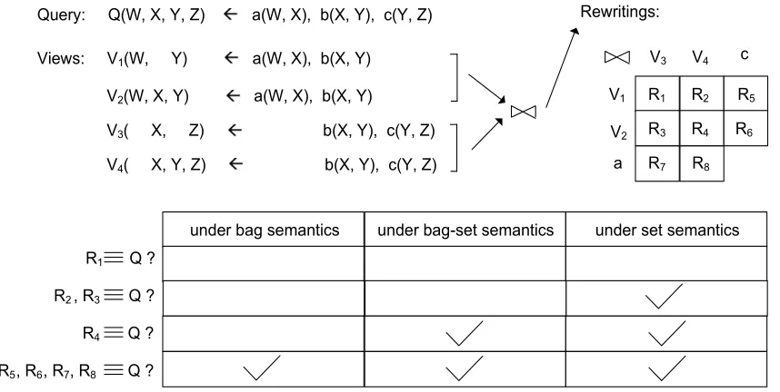
Query: Q(W, X, Y, Z) a(W, X), b(X, Y), c(Y, Z) Views: V1(W, Y) a(W, X), b(X, Y)
V2(W, X, Y) a(W, X), b(X, Y)
V3( X, Z) b(X, Y), c(Y, Z) V4( X, Y, Z) b(X, Y), c(Y, Z)
R1 R2 R3 R4 R6 R7
R5 V1
V2 a
V3 V4 c Rewritings:
under bag-set semantics
under bag semantics under set semantics
R1 Q ? R2, R3 Q ? R4 Q ? , R7, R8 Q ? , R6
R5
R8
Figure 2.2: The equivalence of the rewritings to the query: an example.
2.1.1 Motivations
An important motivation of our work is that under different query semantics we may get different equivalence results for a query and its view-based rewritings.
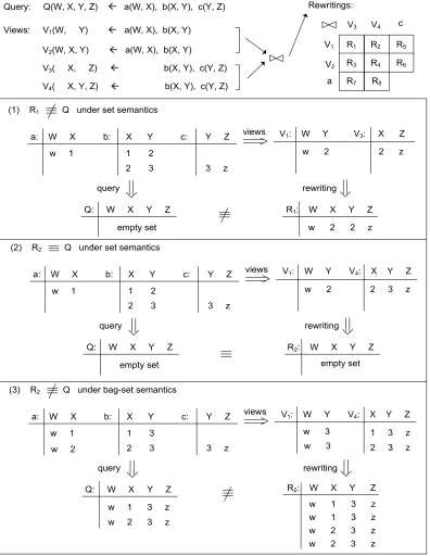
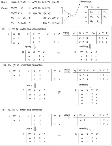
Example 2 In Figure 2.2 there exist multiple possible candidate rewritings of the query, but they have different equivalence properties w.r.t. the given query. For example, R2 and
R3 are equivalent to the query under set semantics only, while R4 is not equivalent to the query only under bag semantics. (Figure 2.3 and Figure 2.4 use specific data instances to illustrate why the rewritings in Figure 2.2 are equivalent or not equivalent to the query.)
More generally, we can get the equivalence relationships between a query and its view-based rewritings under different query semantics as follows.
Lemma 1 Given a query Q and one of its candidate rewritings R, ifR is equivalent toQ
under bag semantics (or under bag-set semantics, respectively), thenR is also equivalent to
Q under bag-set semantics (or under set semantics, respectively).
(1) R1 Q under set semantics
a: W X b: X Y c: Y Z
w 1 1 2
2 3 3 z Query: Q(W, X, Y, Z) a(W, X), b(X, Y), c(Y, Z)
Views: V1(W, Y) a(W, X), b(X, Y)
V2(W, X, Y) a(W, X), b(X, Y)
V3( X, Z) b(X, Y), c(Y, Z)
V4( X, Y, Z) b(X, Y), c(Y, Z)
R1 R2
R3 R4 R6
R7
R5
V1
V2
a
V3 V4 c
Rewritings:
V1: W Y V3: X Z
w 2 2 z views
Q: W X Y Z
empty set
R1: W X Y Z
query rewriting
w 2 2 z
(2) R2 Q under set semantics
a: W X b: X Y c: Y Z
w 1 1 2
2 3 3 z
w 2 2 3 z views
Q: W X Y Z
empty set
R2: W X Y Z
query rewriting
(3) R2 Q under bag-set semantics
a: W X b: X Y c: Y Z
w 1 1 3
2 3 3 z
w 3 views
Q: W X Y Z R2: W X Y Z
query rewriting
w 1 3 z
V1: W Y V4: X Y Z
empty set
w 2 w 3
V1: W Y V4: X Y Z
1 3 z
2 3 z
w 1 3 z
w 2 3 z w 1 3 z w 2 3 z w 2 3 z R8
(4) R4 Q under bag-set semantics
a: W X b: X Y c: Y Z w 1 1 3
2 3 3 z Query: Q(W, X, Y, Z) a(W, X), b(X, Y), c(Y, Z) Views: V1(W, Y) a(W, X), b(X, Y)
V2(W, X, Y) a(W, X), b(X, Y)
V3( X, Z) b(X, Y), c(Y, Z)
V4( X, Y, Z) b(X, Y), c(Y, Z)
R1 R2
R3 R4 R6
R7
R5
V1
V2
a
V3 V4 c
Rewritings:
V2: W X Y V4: X Y Z
w 1 3 w 2 3 views
Q: W X Y Z R4: W X Y Z
query rewriting
(5) R4 Q under bag semantics
(6) R8 Q under bag semantics
w 2
1 3 z 2 3 z
w 1 3 z w 2 3 z
w 1 3 z w 2 3 z a: W X b: X Y c: Y Z
w 1 1 2
1 2 2 z
V2: W X Y V4: X Y Z
w 1 2 w 1 2 views
Q: W X Y Z R4: W X Y Z
query rewriting
1 2 z 1 2 z
w 1 2 z w 1 2 z w 1 2 z w 1 2 z w 1 2 z w 1 2 z
a: W X b: X Y c: Y Z w 1 1 2
1 2 2 z
a: W X V4: X Y Z
w 1 views
Q: W X Y Z R8: W X Y Z
query rewriting
1 2 z 1 2 z
w 1 2 z w 1 2 z w 1 2 z w 1 2 z R8
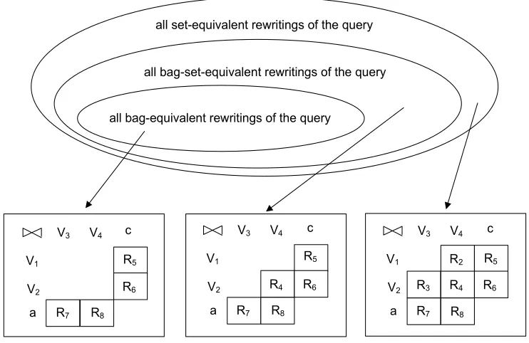
all bag-equivalent rewritings of the query
all bag-set-equivalent rewritings of the query all set-equivalent rewritings of the query
R6 R7
R5 V1
V2 a
V3 V4 c
R4 R6 R7
R5 V1
V2 a
V3 V4 c
R2
R3 R4 R6
R7
R5 V1
V2 a
V3 V4 c
R8 R8 R8
Figure 2.5: The search space of a view-based query optimizer (w.r.t. Figure 2.2).
definitions in Figure 2.1. Based on this lemma, we can describe the search space of a view-based query optimizer in Figure 2.5. That is, the space of all bag-equivalent rewritings of a queryQis contained in the space of all bag-set-equivalent rewritings of Q, which is in turn contained in the space of all set-equivalent rewritings of Q.
As a result, the view-based query optimizer proposed in [17], which explores the space of the bag-equivalent rewritings of the queryQ, is not sufficient for finding the optimal rewritings of Q under bag-set or set semantics. This motivates us to propose new view-based query optimizers to derive the optimal rewriting of the query under bag-set or set semantics.
2.1.2 Contributions
for testing equivalence of queries and rewritings; the algorithm for the set-semantics case builds on results of [28, 29]. (Our algorithms are complete with respect to the language of rewritings — SPJ rewritings for SPJ queries, and central rewritings [26] for queries with aggregation.) Areas where our algorithms are applicable include query optimization, maintenance of physical data independence, and data warehousing.
We propose sound dynamic programming algorithms based on our local conditions, for finding efficient execution plans for user queries using materialized views; queries and views may have grouping and aggregation. Our approach is a relatively simple generalization of the cost-based query-optimization algorithm of [17], which works in an expanded search space of rewritings. While exploring strictly more rewritings than the approach of [17], in general our algorithms for bag-set and set semantics are incomplete; we present a theoretical study of the completeness-efficiency tradeoff and describe enhancements that would make the algorithms complete. Finally, we provide experimental results that show good efficiency and scalability of one of our algorithms for bag-set and set semantics and test the limits of query optimization using overlapping views.
Note that this is joint work with another student Maxim Kormilitsin. In this work, I focus on: (1) exploring equivalent rewritings of the query under set semantics; (2) designing the sub-optimal query optimization algorithm BDPV; (3) developing results for the Select-Project-Join queries, while the work on (4) exploring equivalent rewritings of the query under bag-set semantics and (5) designing the complete query optimization algorithm CDPV and (6) developing results for the aggregate queries with SUM/COUNT/MAX/MIN operators and (7) performance evaluation will be reviewed in Maxim’s thesis [30].
2.2
Preliminaries
In this section we formally review bag, bag-set, and set semantics for query eval-uation, discuss some concepts in answering queries using views, state formally the problem considered in this chapter, and discuss some relevant past work.
2.2.1 Equivalent rewritings and views
We consider SQL Select-Project-Join queries with equality comparisons, possibly with grouping and aggregation, posed on stored (base) relations in a relational database. A relation can be either a set or a bag; a bag can be thought of as a set of elements with multiplicities attached to each element. A database isset-valued if all its base relations are sets, and is bag-valued otherwise.
Two queries Q1 and Q2 are bag-equivalent (Q1 ≡b Q2) if they produce the same
bag of answers on every bag-valued database. Q1andQ2arebag-set-equivalent(Q1≡bs Q2)
if they produce the same bag of answers on every set-valued database. Finally, Q1 and Q2
are set-equivalent(Q1 ≡s Q2) if they produce the same set of answers on every set-valued
database. Chandra and Merlin [31] show that under set semantics, a conjunctive query (CQ) Q1 is contained in a CQ Q2, Q1 ⊑s Q2, if and only if there exists a containment mapping, which maps the head and all the subgoals of Q2 to Q1; the mapping maps each
variable to a single variable or constant, and each constant to the same constant. Q1 and
Q2 are equivalent under set semantics if and only ifQ1⊑sQ2 and Q2⊑sQ1. For bag and
bag-set semantics, the following conditions hold for CQ query equivalence [25]:
Theorem 1 Let Q1 and Q2 be conjunctive queries. (1) Q1 and Q2 are equivalent under
bagsemantics if and only ifQ1 andQ2 are isomorphic. (2)Q1andQ2 are equivalent under
bag-set semantics if and only if Q′
1 and Q′2 are equivalent under bag semantics, where Q′1 and Q′
2 are canonical representations of Q1 and Q2,respectively.1
Aviewrefers to a named query. A viewV is said to bematerializedin a databaseD if its answerV(D) is stored in the database;D{V1,...,Vn} is a databaseDwith added relations for the views V1, . . . , Vn. A rewriting R of a query Q on a set of views V is an equivalent rewriting under set semantics if for every set-valued database D, R(DV) =Q(D), that is,
1QueryQ′is acanonical representationof a queryQifQ′is obtained by removing all duplicate subgoals
R(DV) and Q(D) are the same as sets. The definitions for the bag-set and bag semantics
are analogous. In the rest of the chapter, unless otherwise noted, the term “rewriting” means an “equivalent rewriting” of a query using views, under the semantics specified either explicitly or by the context. We also assume that the definitions of queries and views under consideration are minimized [31]. In practice, user queries and views defined on a database are often already minimized by their creators; in general, we assume that our problem inputs are preprocessed by using well-known minimization algorithms [28, 31].
For a rewriting R of a queryQ using views, we obtain the expansion Rexp of R
by replacing all view atoms in the body ofR by their definitions in terms of base relations. Theorem 2 gives well-known necessary and sufficient conditions for CQ query-rewriting equivalence under each of the three semantics; these conditions follow directly from [18], from Theorem 1, and from straightforward observations on the equivalence of CQ rewritings, in terms of CQ views, to their expansions, under each of the three semantics for query evaluation that we consider.
Theorem 2 For a CQ query Q and a set of CQ views V, let R be a CQ rewriting of Q
using V. Then (1) Q ≡s R iff Rexp ≡s Q on all set-valued databases D; (2) Q ≡b R iff
Rexp≡b Q on all bag-valued databases D; and (3) Q≡bs R iff Rexp≡b Q on all set-valued databases D.
2.2.2 Our problem statement
We now introduce feasible, efficient, and optimal rewritings, give a formal state-ment of our problem, and discuss our assumptions. For a fixed database schema S and given a CQ queryQonS and a set of CQ viewsV defined onS, a CQ queryR is afeasible rewriting of Qfor set, bag-set, or bag semantics X if (1)Ris defined in terms of V, and (2) R is equivalent to Q under the semantics X,R ≡X Q. Efficient rewritings are defined as
follows: Given a databaseD with schemaS, a CQ queryQon D, and a set of CQ viewsV defined on S, a CQ queryR is anefficient rewriting of Qfor set, bag-set, or bag semantics X and given a cost modelM, if (1)R is a feasible rewriting of Q, and (2) the cost of eval-uating R on DV using the cost model M, CM(R, DV), is lower than the cost CM(Q, DV)
of evaluating the query Q in its original formulation. A feasible rewriting R is optimal if CM(R, DV) is minimal among allCM(R′, DV) whereR′is a feasible rewriting ofQforV, X.
Q(a rewriting using views V) is the cost of computing the answer toQusing a lowest-cost query plan for F on DV, for a fixed cost model M. Our problem statement is as follows. Problem 1 Find an optimal CQ rewriting of a minimized [31] CQ queryQ on a database
Dusing minimized CQ viewsV, for set, bag-set, or bag semantics X and given a cost model
M.
All theoretical results in this chapter hold undermonotonic cost models [28]. In-tuitively, a cost model is monotonic if replacing a relation by a smaller relation in — or removing a redundant subgoal from — a query plan never results in higher execution costs; many cost models proposed for and used in query optimization are monotonic (see, e.g., [32]).
Our results in this chapter hold under the following additional assumptions. We consider CQ queries, views, and rewritings of the form described in Section 2.2.1. Further, we allow rewritings that use base relations alongside views (see, e.g., rewritingsR5 through
R8 in Figure 2.2). As the database schema is not part of our problem input, in proving
our complexity results we assume that the number of attributes in each base relation is a constant. For the cases of bag-set and set semantics, we assume that each rewritingR that is equivalent to a query Qcontains no filtering views [28, 18, 29], that is, does not contain views whose removal does not result in loss of equivalence of R to Q. Finally, we assume that a query optimizer considers only left-deep join trees for query plans [17, 32, 24].
2.2.3 View tuples and efficient rewritings
In this chapter we use the results of [28] on restricting the search space of efficient rewritings under set semantics. We first give the definition of a view tuple [28, 18]. Given a queryQ, acanonical database DQ ofQis obtained by turning each subgoal into a tuple by
replacing each variable in the body ofQ by a distinct constant, and treating the resulting subgoals as the only tuples inDQ. LetV(DQ) be the result of applying the view definitions
V on DQ. For each tuple in V(DQ), we restore each new constant back to the original
variable ofQ, and obtain aview tuple of each view with respect to the query. By definition, each variable in each view tuple ofQ occurs in the definition of Q. Let T(DQ) denote the
set of all view tuples after the replacement.
such that R′ is in the form r′( ¯X) ← p1( ¯Y1′), . . . , pk( ¯Yk′), where each pi( ¯Yi′) is a view tuple in T(DQ).
[28] gives examples, for the set-semantics case, of equivalent rewritings whose subgoals are not view tuples.
Theorem 3 Given a database D, a CQ query Q, and a set of CQ views V, under set, bag-set, or bag semantics X and using a monotonic cost model M, consider the set R of all feasible CQ rewritings R of Q in terms of V. Let Ropt ⊆ R be the set of optimal CQ rewritings of Q on D using the cost modelM. Then for at least one rewritingRopt∈ Ropt, each subgoal of Ropt is a view tuple in T(DQ).
Our Theorem 3 holds for conjunctive queries, views, and rewritings both with and without aggregation. The proof of Theorem 3 is immediate from the definition of monotonic cost models (and, for set semantics, from Theorem 5.1 in [28]), after we make the following observation for the cases of bag or bag-set semantics [26, 25, 27]. LetRbe a CQ rewriting of a queryQusing viewsV under bag or bag-set semantics, such that at least one subgoal ofR is not a view tuple inT(DQ). ThenR is not equivalent toQunder the given semantics. In
the remainder of the chapter we consider only rewritings that consist entirely of view tuples (in a broader sense than that of [28], i.e., we also consider view tuples for base relations), for a given query, views, and base relations.
In this chapter we use the notion of tuple core of [28]. Intuitively, given a queryQ and a view tupletV, a tuple core of the view tuple is the maximal set of query subgoals that
can be “covered” by the view tuple in some rewriting of the query. For a formal definition, please see Section 2.3.1. A tuple core is unique for a given pair (Q, tV) [28].
We now restate the bag-semantics part of Theorem 2 using the notion of tuple core.
Proposition 1 Given a CQ queryQon database with schemaS, and given a CQ rewriting
R in terms of CQ viewsV1, . . . , Vm defined onS. Lets1, . . . , sm be the tuple cores of all the view tuplestv1, . . . , tvm in the rewriting R, respectively. ThenQandR are equivalent under bag semantics if and only if (1) all the si’s are pairwise disjoint, (2) the union of all the
Algorithm 1: Query-optimization algorithm CKPS [6] Input : queryQ, table M apT able, cost modelM Output: optimal execution plan forQ w.r.t. M begin
foreach cell Di of P lanT ablein increasing size do foreach (Dj, hj) in MapTable do
if cells Di andDj are disjoint then
AddPlan(Di∪Dj, P =P lanT able[Di]⊲⊳ hj)
//set P as plan for cellDi∪Dj
//if cost(P) is the best so far for that cell
return the plan for the cell for all subgoals ofQ end
2.2.4 Query optimization under bag semantics
The cost-based query-optimization algorithm of [24] uses dynamic programming to find optimal query plans. The approach of [17] (we call it “the CKPS approach”) extends the algorithm of [24] by including view-based query plans into the search space of the optimizer. The CKPS approach uses a preprocessing stage, which determines for each view or base relation V whether V is usable in answering the query and, if so, which subgoals of the queryV “covers.” That is, for each view (or base relation)V which is usable for the query, the preprocessing stage returns all view tupleshj of V and the respective nonempty tuple
cores Dj. The output of this stage is a mapping table called MapTable. The main stage
of the CKPS approach is given as Algorithm 1. Intuitively, the algorithm considers each set of query subgoals as a subproblem (we call it “cell”) in dynamic programming; while the algorithm of [24] finds for each cell an optimal plan in terms of base relations only, the CKPS algorithm also checks whether each cell is “exactly covered” by (i.e., whether each cell is the tuple core of) any view tuple returned by the preprocessing stage and, if so, estimates the cost of evaluating the cell using relevant view tuples. Then the algorithm chooses for the cell one optimal plan from all available (including view-based) plans.
that the CKPS algorithm is sound and complete for CQ queries and views under bag semantics. We use the CKPS approach as the basis of our query-optimization algorithms, see Section 2.4.
2.3
Rewritings: Set Semantics
We now characterize set-equivalence of CQ queries and rewritings. Specifically, we will define a local condition for checking whether two view tuples can be combined in a rewriting that is equivalent to the given query under set semantics. This local condition can help explain why R1 in Figure 2.2 is not set-equivalent to the query whileR2 through
R8 are set-equivalent to the query.
2.3.1 Tuple coverages of view tuples
In this subsection we extend the notion of tuple core of [28] (Section 2.2.3) by defining “tuple coverage.” Intuitively, given a query and a view tuple, a tuple coverage of the view tuple is some set of query subgoals that can be “covered” by the view tuple in some rewriting of the query. Formally, given a CQ queryQ, a CQ rewriting R≡sQ, and a
CQ view V inR, let tV ∈ T(DQ) beV’s view tuple for Q. Then a tuple coverage s(tV, Q)
of tV is a nonempty set G of subgoals of Q, such that (1) G is isomorphic to some set of
subgoals in the expansion texpV of tV, and (2) each variable Y ofG is a head variable oftV
whenever either Y is a head variable of the query Qor Y is used in a subgoal pi( ¯Yi) of Q
such that pi( ¯Yi) is not inG. The tuple core[28], smax(tV, Q), of a view tupletV for query
Qis a tuple coverage that uses a maximal setG of subgoals of Q.
Example 3 The tuple coverages of the view tuples in Figure 2.2 are as follows:
tV1 has exactly one tuple coverage {a, b};
tV2 has three tuple coverages {a, b}, {a}, and{b}; tV3 has exactly one tuple coverage {b, c};
tV4 has three tuple coverages {b, c}, {b}, and{c};
We will see in this section how our approach decides on whether it is possible to combine two view tuples tV and tW in a rewriting that is equivalent to the given query Q
under set semantics; the idea of the approach is to examine tuple coverages s(tV, Q) of tV
respective view tuples. At the same time, under bag-set and bag semantics the only tuple coverages that matter in equivalent rewritings are full tuple cores.
2.3.2 Containment: partition condition
In this subsection we formulate a necessary and sufficient partition condition for combining two view tuples in a rewriting of a CQ query using CQ views under set semantics; this condition gives us a procedure for constructing efficient equivalent rewritings of queries using views.
Intuitively, a queryQis equivalent to a rewritingRif and only if there is a partition of the set of subgoals of Q into subsets, such that each subset Gi is “covered” by a view
tuple for view Vi inR. We now state this result formally, as Theorems 4 [28] and 5.
Theorem 4 Given a CQ query Q on a database with schema S and a set of CQ views
V1, . . . , Vn defined on S, with view tuples tV1, . . . , tVn, respectively. Let a rewriting R use
tV1, . . . , tVn and have the head of Q.Then R contains Q under set semantics, Q⊑sR.
Theorem 5 Given a CQ query Q on a database with schema S and a CQ rewriting R in terms of CQ viewsV1, . . . , Vn defined onS, with view tuplestV1, . . . , tVn, respectively. LetR andQhave the same heads (thusQ⊑s R). ThenR⊑sQ(and therefore R≡s Q) if and only if the set {tVj}of view tuples inR has a subset{t
∗
Vi},i∈ {1, . . . , m}, m≤n,with tuple cov-erages s(t∗Vi, Q), such that the following partition condition holds: (1) s(t∗V
k, Q) T
s(t∗V
l, Q) is an empty set for each k, l ∈ {1, . . . , m} (k6=l), and (2) Si=1m s(t∗Vi, Q) =GQ, where GQ is the set of subgoals of the query Q.
The proof of Theorem 5 is given in the Appendices section (Sections 6.1 and 6.2). We also illustrate this result using the following example.
Example 4 See Figure 2.2. First, R1 = V1 ⊲⊳ V2 is not set-equivalent to Q, since the only tuple coverage oftV1,{a, b} (see Example 3), and the only tuple coverage of tV2,{b, c},
overlap on the subgoal b. Second, R2 =V1 ⊲⊳ V4 is set-equivalent to Q, since the only tuple coverage of tV1, {a, b}, and one of the three tuple coverages of tV4, {c}, form a partition
2.3.3 Efficient algorithm for partition checking
We now present an E-MCD-Partition algorithm for checking the partition condi-tion of Theorem 5 under set semantics, for CQ queries, views, and rewritings. The algo-rithm has been inspired by MiniCon Descriptions (MCDs), developed in [29] in the context of computing maximally contained rewritings. We adapt MCDs to our context of equivalent rewritings, by defining anE-MCD for a given view tupletV of a CQ view V on CQ query
Q as a minimal tuple coverage of tV. That is, an E-MCD is any tuple coverage s(tV, Q)
of tV on Q, such that no proper subset of subgoals of s(tV, Q) is also a tuple coverage of
tV on Q. (In Example 3, {a, b} is the only E-MCD of tV1 and {b, c} is the only E-MCD of tV3, whereas tV2 has two E-MCDs,{a} and{b}, andtV4 has two E-MCDs,{b}and {c}.) It is easy to see that, given a CQ query Q and a view tuple tV for a CQ view V, the set of
all E-MCDs of tV on Q provides a partition of the tuple core of tV on Q. There exists a
quadratic-time procedure for finding all E-MCDs of a view tuple for a query.
Our algorithm E-MCD-Partition is based on an equivalent rephrasing of Theo-rem 5, which replaces “tuple coverages” by “sets of E-MCDs.” E-MCD-Partition operates on exactly two view tuples. We give a pseudocode for E-MCD-Partition as Algorithm 3, which includes a preprocessing step as described in Algorithm 2.
Pre-processing (Algorithm 2):
Algorithm 2 mainly includes two steps. (1) Lines 1-7: Find all neighbors of each E-MCD oftv (tw). Here a neighbor of a E-MCD Mi oftv (tw) is an E-MCDMj oftw (tv)
that overlaps with Mi on at least a subgoal. (2) Lines 8-15: Classify all E-MCDs of tv and
tw into three classes: EXCLUSIVE (line 9), SHARED (line 10), and CROSSOVER (line
11).
Example 5 Given two view tuples V and W as follows, where each si is a subgoal and
each ‘[ ]’ represents an E-MCD. V: [s1,s2] [s3,s4] [s5, s6] [s7,s8]
W: [s4,s5] [s6,s7] [s8,s9] [s10,s11]
Next we represent each ‘[ ]’ using a correspondingMi. Then, we have
V: M1,M2,M3,M4
W: M5,M6,M7,M8
Algorithm 2: Procedure: pre-processing()
Input : two view tuples tv and tw and their E-MCDs
//Construct one bucket for each subgoal foreach E-MCDMi of tv and tw do
1
foreach subgoal sk inMi do
2
Bucket(sk) = Bucket(sk) ∪ {Mi};
3
//Find the overlapping E-MCDs oftv and tw foreach subgoalsk do
4
if |Bucket(sk)|= 2then
5
// Bucket(sk) has two E-MCDs: Mi from tv and Mj from tw
Mi.neighbors =Mi.neighbors∪ {Mj};
6
Mj.neighbors = Mj.neighbors ∪ {Mi};
7
//Classify all E-MCDs of tv and tw foreach E-MCDMi of tv (tw) do
8
if no subgoals inMi appear intw (tv) then Mi.type = EXCLUSIVE;
9
else if all subgoals inMi appear intw (tv) then Mi.type = SHARED;
10
else Mi.type = CROSSOVER;
11
ALLV ← all of t
v’s E-MCDs;
12
EXCLU SIV EV ← all of t
v’s EXCLUSIVE-type E-MCDs;
13
SHAREDV ←all of t
v’s SHARED-type E-MCDs;
14
CROSSOV ERV ← all oftv’s CROSSOVER-type E-MCDs;
15
//The above definitions w.r.t. v also applies similarly tow
M2.neighbors = {M5};
M3.neighbors = {M5, M6};
M4.neighbors = {M6, M7};
M5.neighbors = {M2, M3};
M6.neighbors = {M3, M4};
M7.neighbors = {M4};
M8.neighbors = φ;
EXCLU SIV EV = {M1};
CROSSOV ERV ={M 2};
SHAREDV ={M 3, M4};
ALLW ={M5, M6, M7, M8};
EXCLU SIV EW ={M8};
CROSSOV ERW = {M7};
SHAREDW ={M5, M6};
We now analyze the time complexity of Algorithm 2. We denote the number of subgoals in each view tuple by O(n) and the number of E-MCDs of each view tuple by O(e). Then, we can see that the time cost of Lines 1-3 is O(n+e), the time cost of Lines 4-7 is O(n+e), the time cost of lines 8-11 is O(n+e), and the time cost of Lines 12-15 is O(e). Therefore, we have the following lemma.
Lemma 3 The time complexity of Algorithm 2 is O(n+e).
E-MCD-Partition(Algorithm 3):
The basic idea of Algorithm 3 is iteratively finding (1) the E-MCDsSiV oftV that
must be used in the final partition (if any); (2) the E-MCDs SiW of tW that must not be
used in the final partition (if any). Specifically, Algorithm 3 works as follows.
Step 1: Initially, we haveS1V =CROSSOV ERV (line 2). Since the CROSSOVER-type E-MCDs oftv have some subgoals that cannot be covered by any E-MCDs oftw, these
CROSSOVER-type E-MCDs of tv must be used in the final partition.
Step 2: Then, we derive S1W, which are the neighbor E-MCDs (in tw) of the
E-MCDs in S1V (line 10). Since the E-MCDs in S1W overlap with the E-MCDs in S1V, which must be used in the final partition, the E-MCDs in S1W must not be used in the final partition.
Step 3: Then, we deriveS2V, which are the neighbor E-MCDs (intv) of the E-MCDs
in SW
1 (line 17). Since the E-MCDs inSV2 overlap with the E-MCDs in S1W, which must
not be used in the final partition, the E-MCDs inSV
2 must be used in the final partition.
Similarly, we can continue this process iteratively to get S2W, S3V, S3W, S4V, S4W, ...
Algorithm 3: E-MCD-Partition
Input : two view tuples tv and tw and their E-MCDs Output: true or false
pre-processing(); (Algorithm 2) 1
// SV aret
v’s E-MCDs that must be used in the final partition (if any);
SV1 ← CROSSOV ERV; 2
// SW aretw’s E-MCDs that must not be used in the final partition (if any)
SW1 ← φ; 3
i= 1; 4
whiletrue do 5
if SV
i =φthen
6
return true;// an E-MCD partition has been found, which are 7
// EXCLU SIV EV ∪(S1V ∪S2V ∪...∪SiV) fromtv
// ALLW −(S1W ∪S2W ∪...∪SiW) fromtw
SW
i ← φ;
8
foreach E-MCDMj inSiV do
9
SiW ←SWi ∪ Mj.neighbors;
10
foreach E-MCDMk inMj.neighborsdo
11
Mk.neighbors← Mk.neighbors− {Mj};
12
Si+1V ← φ; 13
foreach E-MCDMj inSiW do
14
if Mj.type = CROSSOVERthen
15
return false; 16
// Reason: Since Mj is in SiW, it can not be used in the final
// partition. As a result, those subgoals in Mj of tw
// but not in tv cannot be covered by tv ortw !
Si+1V ← Si+1V ∪ Mj.neighbors;
17
foreach E-MCDMk inMj.neighborsdo
18
Mk.neighbors← Mk.neighbors− {Mj};
19
(1) Returnfalse(lines 15-16): In the iteration process, if an E-MCDMj inSWi is
CROSSOVER-type, then we know that there must not exist an E-MCD partition w.r.t. tv
and tw. The reason is, since Mj is in SiW, it cannot be used in the final partition. On the
other hand, sinceMj is CROSSOVER-type, it includes some subgoals that are not covered
by any E-MCDs oftv. Therefore, there must not exist any E-MCD partition that can cover
such subgoals.
(2) Returntrue(lines 6-7): In the iteration process, ifSiV is empty, then we know that we have found an E-MCD partition, which is composed of
E-MCDs fromtv: Pv=EXCLU SIV EV ∪(S1V ∪S2V ∪...∪SiV)
E-MCDs fromtw: Pw =ALLW −(S1W ∪S2W ∪...∪SWi )
since we have the following lemma. (See the Appendices section−Section 6.3 for the proof.) Lemma 4 (a) The E-MCDs inPv andPw do not overlap with each other; (b) The E-MCDs in Pv and Pw together cover all subgoals in tv and tw.
Example 6 Here we continue Example 5. The run-time process of Algorithm 3 is as fol-lows.
Initially, S1V ={M2}; S1W =φ;
1st iteration: S1W = {M5}; S2V = {M3}; 2nd iteration: SW
2 ={M6}; S3V ={M4}; 3rd iteration: SW
3 ={M7}; sinceM7.type = CROSSOV ER, Algorithm 3 returns
f alse, i.e., there does not exist any E-MCD partition w.r.t. V and W.
On the other hand, if we change M7 from {s8, s9} to {s8}, then the run-time process of Algorithm 3 will be as follows.
Initially, S1V ={M2}; S1W =φ; 1st iteration: SW
1 = {M5}; S2V = {M3}; 2nd iteration: SW
2 ={M6}; S3V ={M4}; 3rd iteration: SW
3 = {M7}; S4V =φ;
4th iteration: Since S4V = φ, Algorithm 3 returns true, i.e., at this time we have found an E-MCD partition w.r.t. V and W, which is
EXCLU SIV EV ∪S1V ∪S2V ∪S3V = {M1, M2, M3, M4} from V
ALLW −SW1 ∪S2W ∪S3W = {M8} fromW
tuple by O(e). Then, we can see that the time cost of Line 1 is O(n+e) (Lemma 3), the time cost of Lines 2-4 is O(1), and the time cost of Lines 5-20 is O(e2) (since each of O(e)
E-MCDs is accessed at most once, and then itsO(e) neighbor E-MCDs are accessed). (Note that the time cost of all lines, except for Line 1, in Algorithm 3, is independent on n, and depends oneonly, because these lines operate only on E-MCDs but not on subgoals of view tuples.) Therefore, we have the following lemma.
Lemma 5 The time complexity of Algorithm 3 is O(n+e2). Since eis bounded by n, the time complexity of Algorithm 3 can also be expressed as O(n2).
Therefore, checking the E-MCD partition w.r.t. two views can be done in polyno-mial time. However, the more general problem of checking the E-MCD partition w.r.t. m views (m >2) is much harder, which in fact is NP-Complete, since this problem is polynomi-ally equivalent to the classicExact Coverproblem, which is well known to be NP-Complete. The Exact Cover problem is described as follows [33]: Given a setX and a collection S of subsets of X, find an exact cover S∗ such that S∗ is a subcollection ofS and every element
inXis contained in exactly one set in S∗. It is easy to see that the set of all subgoals of all view tuples in our E-MCD-Partition problem corresponds to the setX in the Exact Cover problem, while the set of all E-MCDs of all view tuples in our E-MCD-Partition problem corresponds to the collection S in the Exact Cover problem (since each E-MCD of a view tuple in our E-MCD-Partition problem corresponds to a subset of X in the Exact Cover problem).
For avoiding such high computational overhead of checking the E-MCD partition w.r.t. mviews (m >2), we take a heuristic strategy, which works in an incremental way that is essential in our following view-based query optimization algorithm BDPV (Section 2.4.1). In this incremental strategy, given m views V1 through Vm, we first check whether there
exists an E-MCD partition w.r.t. V1 and V2 by calling our E-MCD-Partition algorithm in
Algorithm 3. If not, the incremental strategy terminates here and returns false. Otherwise, we can view the set of E-MCDs found in Algorithm 3, which forms an E-MCD partition w.r.t. V1 and V2, as a new ‘view’ V12, and then Algorithm 3 is called again to check
whether there exists an E-MCD partition w.r.t. V12andV3. Similarly, Algorithm 3 is called
iteratively to check the E-MCD partition w.r.t. V123andV4, and then the E-MCD partition
2.4
Cost-Based Query Optimizers for Bag-Set and Set
Se-mantics
When looking for an efficient view-based execution plan for a given CQ query, the dynamic-programming optimization algorithm CKPS of [17] (Section 2.2.4) considers all combinations of view tuples with each other and with base relations, such that the respective tuple cores “do not overlap” — that is, all pairwise intersections of the tuple cores are empty; see, for instance, rewriting R5 through R8 in Figure 2.5. To be able
to produce additional view-based query plans under bag-set and set semantics, such as rewritings R2 through R4 in Figure 2.5, we look for simple efficient local conditions on
combining, in a partial rewriting, view tuples whose tuple cores do overlap.
2.4.1 Basic DP algorithm BDPV
Our basic DP algorithm with views (BDPV) is the CKPS algorithm of [17] en-hanced by processing view tuples with overlapping tuple cores. The preprocessing step of BDPV is exactly the same as that of CKPS; the pseudocode for the main stage of BDPV is shown as Algorithm 4. Just like the main stage of the CKPS algorithm, BDPV consid-ers each set of query subgoals as a subproblem, or “cell,” in dynamic programming, and checks whether each cell is “exactly covered” by any view tuple returned by the prepro-cessing stage. Then BDPV chooses for each cell one optimal plan from all the available — including view-based — plans.
The only difference between CKPS and BDPV is theGoodNontrivialOverlap seg-ment in Algorithm 4. Intuitively, at each DP cell we try to ensure that the partial rewriting we are building is contained in some part of the queryQ. In the GoodNontrivialOverlap segment, after deciding on an optimal plan Pi = P lanT able(Di) for a cell Di of a query
Q, BDPV additionally checks whether the set SDi of base relations (if any) and views (if
any) in the planPi can be combined with each view tupletV whose tuple coresmax(tV, Q)
“nontrivially overlaps” with the set of query subgoals Di. Then, for each view tuple tV
that can be successfully combined with a cell plan Pi (with tuple core Di), BDPV adds
the resulting combination to the set of candidate plans for the DP cell whose set of query subgoals is exactly the union of the tuple cores oftV and Pi. For instance, for the example
Algorithm 4: Query-optimization algorithm BDPV Input : queryQ, table M apT able, cost modelM Output: optimal execution plan forQ w.r.t. M begin
foreach cell Di of P lanT ablein increasing size do
1
foreach (Dj, hj) in MapTable do
2
if cells Di andDj are disjoint then
3
AddPlan(Di∪Dj, P =P lanT able[Di]⊲⊳ hj)
4
//set P as plan for cellDi∪Dj
//if cost(P) is the best so far for that cell
else 5
if GoodNontrivialOverlap(P lanT able[Di], Dj) == truethen
6
AddPlan(Di∪Dj, P lanT able[Di]⊲⊳ hj)
7
return the plan for the cell for all subgoals ofQ 8
end
queryQthe combinations of view tuples, (V1, V4) (i.e.,R2), (V2, V3) (i.e., R3), (V2, V4) (i.e.,
R4), and so on (but not (V1, V3) (i.e., R1)).
We now give an outline of this additional processing in BDPV, by first defining the nontrivial-overlap condition and then describing the combination test, that is, necessary and sufficient conditions for combining view tuples with partial query plans. We say that two sets s1 and s2 of subgoals of query Q nontrivially overlap if (1) the intersection of s1
and s2 is nonempty, as is (2) each of the sets s1−s2 and s2−s1. Intuitively, condition
(1) provides the “overlap,” whereas (2) ensures that each of s1 and s2 contributes to the
combination some query subgoals that the other set does not. (Recall that our monotonic cost models discourage rewritings with redundant base-relation or view subgoals.)
We now describe the combination test that BDPV does. Consider a DP cell Di
and the combination SDi of base relations and views in an optimal planPi forDi; suppose
tV is a view tuple whose tuple core smax(tV, Q) nontrivially overlaps with the set of query
![Figure 3.6: LF: Incorrect order of calling blocks (query: ‘//*[//A]/B/C’).ö from seeing its own copy in is read,](https://thumb-us.123doks.com/thumbv2/123dok_us/1395807.1172286/60.612.113.532.91.396/figure-incorrect-order-calling-blocks-query-seeing-copy.webp)