Solid-State NMR of Quadrupolar Nuclei for Structural Elucidation

University of Windsor University of Windsor

Scholarship at UWindsor

Scholarship at UWindsor

Electronic Theses and Dissertations Theses, Dissertations, and Major Papers

2012

Solid-State NMR of Quadrupolar Nuclei for Structural Elucidation

Solid-State NMR of Quadrupolar Nuclei for Structural Elucidation

Marcel Hildebrand University of Windsor

Follow this and additional works at: https://scholar.uwindsor.ca/etd

Recommended Citation Recommended Citation

Hildebrand, Marcel, "Solid-State NMR of Quadrupolar Nuclei for Structural Elucidation" (2012). Electronic Theses and Dissertations. 305.

https://scholar.uwindsor.ca/etd/305

This online database contains the full-text of PhD dissertations and Masters’ theses of University of Windsor students from 1954 forward. These documents are made available for personal study and research purposes only, in accordance with the Canadian Copyright Act and the Creative Commons license—CC BY-NC-ND (Attribution, Non-Commercial, No Derivative Works). Under this license, works must always be attributed to the copyright holder (original author), cannot be used for any commercial purposes, and may not be altered. Any other use would require the permission of the copyright holder. Students may inquire about withdrawing their dissertation and/or thesis from this database. For additional inquiries, please contact the repository administrator via email

Solid-State NMR of Quadrupolar Nuclei for Structural Elucidation

by

Marcel P. Hildebrand

A Thesis

Submitted to the Faculty of Graduate Studies through Chemistry and Biochemistry in Partial Fulfillment of the Requirements for the

Degree of Master of Science at the University of Windsor

Windsor, Ontario, Canada 2012

iii Declaration of Co-Authorship

I acknowledge that my supervisor, Dr. Robert Schurko, has provided guidance

throughout the whole of this work and has edited this thesis.

Dr. Victor Terskikh and Dr. Eric Ye at the National Ultra-high Field NMR

Facility for Solids are acknowledged for providing data acquired at 21.1 T in Chapter 2.

Dr. Ivan Hung and Dr. Zhehong Gan at the National High Magnetic Field Laboratory are

acknowledged for providing the data acquired at 21.1 T in Chapter 3.

Senior members of our lab group trained me in the use of our NMR spectrometer

and supervised my usage of it. The main contributors in this regard were Dr. Aaron

Rossini (Chapter 2), Dr. Hiyam Hamaed (Chapter 3), and Bryan Lucier (Chapter 2 and

3). Other senior graduate students in the Department of Chemistry and Biochemistry

trained me in the use of some synthetic chemistry techniques. The main contributors are

Dr. Jillian Hatnean and Meghan Doster (Chapter 2).

I am aware of the University of Windsor Senate Policy on Authorship and I

certify that I have properly acknowledged the contribution of other researchers to my

thesis, and have obtained written permission from each of the co-author(s) to include the

above material(s) in my thesis. I certify that, with the above qualification, this thesis, and

the research to which it refers, is the product of my own work.

I declare that, to the best of my knowledge, my thesis does not infringe upon

anyone’s copyright nor violate any proprietary rights and that any ideas, techniques,

quotations, or any other material from the work of other people included in my thesis,

iv

referencing practices. Furthermore, to the extent that I have included copyright material

that surpasses the bounds of fair dealing within the meaning of the Canada Copyright

Act, I certify that I have obtained a written permission from the copyright owner(s) to

include such materials in my thesis.

I declare that this is a true copy of my thesis, including any final revisions, as

approved by my thesis committee and the Graduate Studies office, and that this thesis has

v Abstract

This thesis demonstrates that solid-state NMR (SSNMR) spectroscopy of

quadrupolar nuclei provides a powerful means of characterizing a diverse set of

materials. Complementary techniques such as pXRD and quantum chemical calculations

are also explored.

First, information on the structure and function of methylalumoxane (MAO) is

obtained via 27Al and 91Zr SSNMR experiments at two different magnetic field strengths.

In particular, 27Al NMR and accompanying first principles calculations reveal the nature

of the Al sites in the cage-like MAO structures, and lend insight into the interactions that

lead to the formation of the MAO/metallocene adducts.

Second, a series of hydrochloride (HCl) pharmaceuticals are characterized via

35

Cl SSNMR, and arrangements of close-contact hydrogen bonds are correlated to 35Cl

EFG tensor parameters. Plane-wave density functional theory calculations of these

parameters are in good agreement with experiment. 35Cl SSNMR is also shown to act as

vi Acknowledgements

Many thanks go to my supervisor, Dr. Robert Schurko, for providing guidance as

I undertook the study of solid-state NMR. This area of research is a difficult one and Rob

has guided me the entire way. I have not only learned about SSNMR, but more

importantly, I have learned how to be a critical thinker in addition to many other skills

that I will keep with me for a lifetime. For that I thank you.

Thanks also to Dr. Loeb and Dr. Rangan for being on my M.Sc. thesis committee

and agreeing to read through this work. Dr. Gauld is thanked for chairing my defense.

I also acknowledge all the members of the Schurko group past and present: Dr.

Karen Johnston, Dr. Kris Harris, Dr. Aaron Rossini (whom I expect to see in an academic

faculty position soon), Dr. Hiyam Hamaed, Dr. Luke O’Dell, Bryan Lucier, Stanislav

Veinberg, Andrew Namespetra, Zach Friedl, and Chris O’Keefe. Thanks for the help and

some great discussions.

Thanks to Karla Day. You have always been supportive of me and my decisions,

in spite of my ‘flaky’ and unpredictable behavior. You are my favorite person and I can

only hope to be there for you as you have been there for me. May you walk on warm

sands.

Lastly, I would like to thank my family. Your support and encouragement is

appreciated, despite living on opposite sides of the country. You have all taught me the

vii Contents

Declaration of Co-Authorship...iii

Abstract...v

Acknowledgements... vi

List of Tables... xi

List of Figures... xiv

List of Abbreviations... xxiii

List of Symbols... xxv

1 Introduction and Theory ...1

1.1 Introduction... 1

1.2 NMR Interactions...2

1.2.1 Zeeman Interaction...2

1.2.2 Response of Nuclear Spins to Radiofrequency Pulses...6

1.2.3 Relaxation Processes... 8

1.2.4 Nuclear Shielding and the Chemical Shift... 9

1.2.5 Quadrupolar Interaction...15

1.2.6 Euler Angles...21

1.2.7 Dipolar and Scalar Coupling... 22

1.3 NMR Acquisition and Signal Enhancement Techniques...25

1.3.1 Magic-Angle Spinning (MAS)...25

1.3.2 Echo Pulse Sequences... 28

1.3.3 Frequency-stepped SSNMR...30

viii

1.3.5 Cross Polarization...33

1.3.6 Multiple-Quantum Magic-Angle Spinning (MQMAS)...35

1.3.7 Quantum Chemical Calculations of NMR Tensor Parameters...38

1.4 Context of Research... 39

Bibliography...41

2 Multinuclear NMR Spectroscopy of Methylalumoxane: Solid Forms of the Co-catalyst and Metallocene Adducts...48

2.1 Introduction... 48

2.2 Experimental...56

2.2.1 Samples...56

2.2.2 Solid-State NMR... 56

2.2.3 Theoretical Calculations...59

2.3 Results and Discussion...60

2.3.1 General Overview...60

2.3.2 27Al SSNMR experiments, MAO...60

2.3.3 27Al SSNMR experiments, MAO and Cp2ZrMe2/MAO adducts...65

2.3.4 27Al MQMAS Experiments. MAO and Cp2ZrMe2/5MAO...74

2.3.5 First principles calculations of 27Al EFG tensors...78

2.3.6 91Zr SSNMR experiments, Cp2ZrMe2/MAO adducts... 80

2.4 Conclusions...84

ix

3 Combining 35Cl Solid-State NMR and First Principles DFT Calculations for the Study of HCl Pharmaceuticals and their

Polymorphs...96

3.1 Introduction... 96

3.2 Experimental...101

3.2.1 Samples...101

3.2.2 Solid-State NMR (9.4 T)...101

3.2.3 Solid-State NMR (21.1 T)...102

3.2.4 Powder XRD... 103

3.2.5 Theoretical Calculations...103

3.3 Results and Discussion...104

3.3.1 General Overview... 104

3.3.2 Reliability of Plane-Wave DFT Calculations...105

3.3.3 A system with one short H···Cl contact: Dicyclomine HCl (Dicy)...110

3.3.4 Systems with two short H···Cl contacts: Nylidrin HCl (Nyli), Scopolamine HCl (Scop) and Bromhexine HCl (Brom)... 112

3.3.5 Systems with three short H···Cl contacts: Alprenolol HCl (Alpr), Isoprenaline HCl (Isop), and Procainamide HCl (Proc)...115

3.3.6 Systems with four or more short H···Cl contacts: Dopamine HCl (Dopa) and Aminoguanidine HCl (Amin)...120

3.3.7 Correlation of chlorine environments and EFG tensor parameters...123

3.3.8 Application to polymorphism in HCl pharmaceuticals...125

3.4 Conclusions...135

x

4 General Conclusions and Future Work...145

Appendices A Supporting Information - Multinuclear NMR Spectroscopy of Methylalumoxane: Solid Forms of the Co-catalyst and Metallocene Adducts...148

A.1 Supporting Experimental Information...148

A.1.1 Experimental Parameters for SSNMR Experiments...148

A.1.2 DFT Calculations of 27Al EFG Tensor Parameters...156

A.1.3 Supplementary Figures and SSNMR Spectra...165

Bibliography...170

B Supporting Information - Combining 35Cl Solid-State NMR and First Principles DFT Calculations for the Study of HCl Pharmaceuticals and their Polymorphs... 171

B.1 Supporting Experimental Information...171

B.1.1 Experimental Polymorph Generation...171

B.1.2 Experimental Parameters for SSNMR Experiments...172

B.1.3 Experimental 35Cl EFG and CSA Tensor Parameters and Short Cl···H Contact Distances and Angles...179

B.1.4 Supplementary Figures... 182

Bibliography...201

xi List of Tables

Table 2.1. Experimentally determined 27Al EFG tensor NMR parameters

for MAO...62

Table 2.2. Experimentally determined 27Al NMR tensor parameters

for MAO...63

Table 2.3. Experimentally determined 27Al EFG tensor parameters for

Cp2ZrMe2/5MAO... 69

Table 2.4. Experimentally determined 27Al NMR tensor parameters for

Cp2ZrMe2/5MAO... 70

Table 2.5. Relative integrated intensities of Sites A, B and C in the

Cp2ZrMe2/MAO adducts at 9.4 T... 71

Table 2.6. Experimentally determined 27Al EFG tensor NMR parameters (21.1 T) for bulk MAO and Cp2ZrMe2/5MAO obtained from

MQMAS cross-sections... 77

Table 2.7. Experimentally determined 91Zr static EFG and CSA tensor NMR parameters for Cp2ZrMe2/5MAO, Cp2ZrMe2, and

[Cp2ZrMe][MeB(C6F5)3] (21.1 T)...83

Table 3.1. Experimental and theoretical 35Cl EFG and CS

tensor parameters...108

Table 3.2. Short H···Cl contacts and experimentally determined 35Cl SSNMR parameters for HCl pharmaceuticals with one and two

close H···Cl contacts...111

Table 3.3. Short H···Cl contacts and experimentally determined 35

Cl SSNMR parameters for HCl pharmaceuticals with three close

H···Cl contacts... 116

Table 3.4. Short H···Cl contacts and experimentally determined 35Cl SSNMR parameters for HCl pharmaceuticals with four or more close

H···Cl contacts... 121

Table 3.5. Short H···Cl contacts and experimentally determined 35Cl

xii

Table 3.6. Experimental and theoretical 35Cl EFG and CS tensor parameters

for HCl pharmaceutical polymorphs... 129

Table A1. Details of Compounds A – G...148

Table A2. SSNMR Acquisition parameters for static 27Al spectra (9.4 T)...149

Table A3. SSNMR Acquisition parameters for static 27Al spectra (21.1 T)...150

Table A4. SSNMR Acquisition parameters for MAS 27Al spectra (21.1 T)...151

Table A5. SSNMR Acquisition parameters for 1H →13C VACP spectra (9.4 T)...152

Table A6. SSNMR Acquisition parameters for MAS 1H spectra (9.4 T)...153

Table A7. SSNMR Acquisition parameters for static 91Zr spectra (21.1 T)...154

Table A8. SSNMR Acquisition parameters for 27Al MQMAS spectra (21.1 T)...155

Table A9. Calculated 27Al EFG tensor parameters for MAO (proposed structures)... 156

Table B1. SSNMR Acquisition parameters for static 35Cl spectra (9.4 T) of Proc, Dicy, Alpr, Isop, Nyli, Dopa, Brom...172

Table B2. SSNMR Acquisition parameters for static 35Cl spectra (9.4 T) of Scop, Amin, Chlo, IsoxI, MexiI, MexiII...173

Table B3. SSNMR Acquisition parameters for static 35Cl spectra (21.1 T) of of Proc, Dicy, Alpr, Isop, Nyli, Dopa, Brom... 174

Table B4. SSNMR Acquisition parameters for static 35Cl spectra (21.1 T) of Scop, Amin, Chlo, IsoxI, MexiI...175

Table B5. SSNMR Acquisition parameters for MAS 35Cl spectra (21.1 T) of Proc, Dicy, Alpr, Isop, Nyli, Dopa, Brom... 176

Table B6. SSNMR acquisition parameters for MAS 35Cl spectra (21.1 T) of Scop, Amin, Chlo, IsoxI, MexiI...177

xiii

Table B8. Experimental 35Cl EFG and CSA tensor parameters... 179

Table B9. Short Cl···H contact distances and angles for HCl

pharmaceuticals containing two hydrogen close contacts...180

Table B10. Short Cl···H contact distances and angles for HCl pharmaceuticals

xiv List of Figures

Figure 1.1. Depiction of nuclear spin angular momentum precessing

about the magnetic field... 4

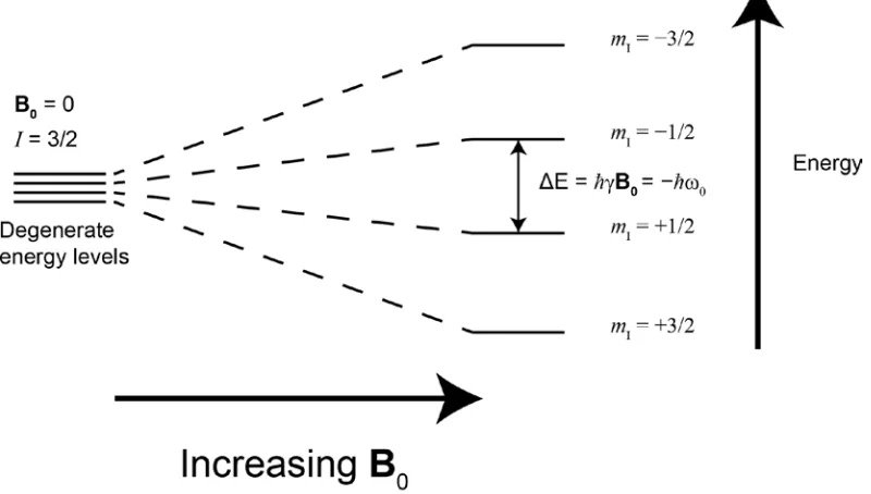
Figure 1.2. Quantization of the nuclear spin angular momentum for I = 3/2 nucleus in the presence of a magnetic field. Note the energy separation between adjacent spin states is equivalent, resulting in a single transition

frequency...5

Figure 1.3. (a) Vector model representation of the effect of a pulse applied along the x′-axis of the rotating frame on the bulk magnetization vector M.

(b) After B1 is turned off, the vector undergoes free precession about B0... 8

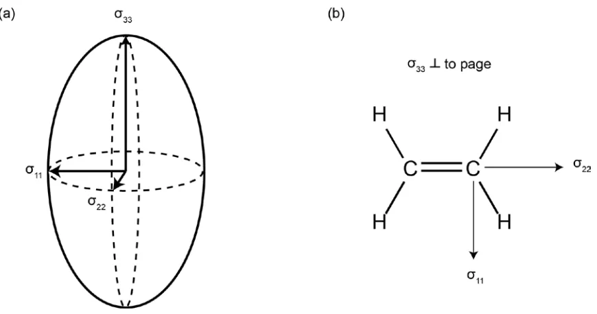
Figure 1.4. (a) Depiction of nuclear shielding tensor orientation with corresponding principal axis components. (b) Nuclear shielding tensor orientation for the carbon atom in ethene. Note the orientation dependence

of the nuclear shielding interaction... 13

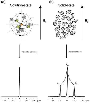
Figure 1.5. (a) Rapid molecular tumbling in solution serves to average the CSA to its isotropic value which, in turn, results in a sharp peak at the

isotropic frequency shift, δiso. (b) Simulated 13C (I = 1/2) static spectrum. The discontinuities correspond to the principal components of the CS tensor.

Note the sharp peaks corresponding to δ11, δ22and δ33, which illustrate how different orientations of the CS tensor, with respect to B0, give rise to distinct transition frequency shifts. In a powdered sample, all orientations

are present, giving rise to a powder pattern...16

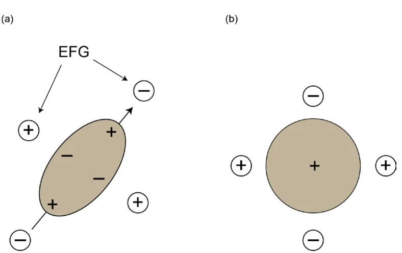
Figure 1.6. (a) Schematic representation of the asymmetric charge distribution for a quadrupolar nucleus and the associated preferential orientation, or interaction, with an electric field gradient. (b) Schematic representation of an I = 1/2 nucleus with a spherical charge distribution. Here there is no preferred orientation with respect to the electric field

gradient...17

Figure 1.7. Perturbation of the Zeeman energy levels arising from the quadrupolar interaction to a first- and second-order approximation for a spin I = 3/2 system. Although not broadened by the first-order quadrupolar interaction, the central transition is broadened by the second-order quadrupolar interaction. The satellite transitions are affected by both the first-and

second-order quadrupolar interaction...20

xv

ηQ ranging from 0.2 to 1.0. The broadening of the powder pattern due to the increased value of CQ, as well as the position of the discontinuities due to ηQ,

are illustrated... 21

Figure 1.9. Depiction of the Euler angle convention used to describe the relative orientation ofthe CS and EFG tensor by rotating the CS tensor from the fixed EFG tensor frame (denoted by the x, y, z frame) into the PAS of the

CS tensor (denoted by the X, Y, Z frame). Adapted from Tang (2008)... 22

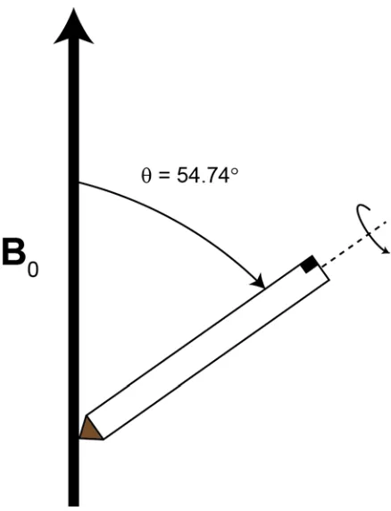
Figure 1.10. Schematic representation of a rotor at the magic-angle of

θ = 54.74° where θ is the angle of the rotor with respect to B0...26

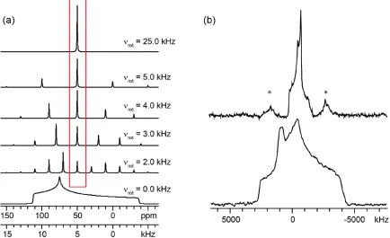
Figure 1.11. (a) Simulated spectra illustrating the effect of MAS on an I = 1/2 powder pattern at various spinning speeds. The isotropic peak is enclosed in the red box. Note the spinning sidebands are offset from the isotropic peak by an integer multiple of the spinning speed.

(b) I = 3/2 MAS (top) and static (bottom) spectra 35Cl SSNMR spectra

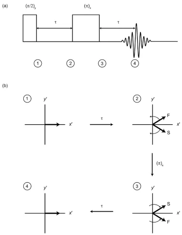
of dopamine HCl. νrot = 22 kHz. Spinning sidebands denoted by *... 27 Figure 1.12. (a) A schematic representation of the Hahn echo pulse

sequence and (b) a vector model illustrating the refocusing of two

representative spins... 29

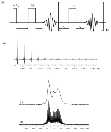
Figure 1.13. (a) A schematic representation of the QCPMG pulse sequence. The parameters τ1, τ2, τ3, and τ4 indicate interpulse delays. (b) An example of the spikelet FID obtained from a 27Al (I = 5/2) QCPMG experiment on methylaluminoxane. (c) Fourier transformation of the first spin echo gives a standard spin echo spectrum. (d) Fourier transformation of the QCPMG

echo train gives a spikelet spectrum...32

Figure 1.14. A schematic representation of the WURST-QCPMG pulse sequence. The parameters τ1, τ2, τ3, and τ4 indicate interpulse delays. The

excitation and refocusing pulses have identical lengths and phases... 33

Figure 1.15. A schematic representation of the cross-polarization pulse sequence. I corresponds to the nucleus with favorable NMR properties (abundant) and S corresponds to the nucleus with unfavorable

NMR properties (dilute)... 34

xvi

projections for RbNO3, recorded using the pulse sequence in (a).

This pulse sequence was not utilized in this study...35

Figure 1.17. Schematic representation of a spectrum resulting from an MQMAS experiment. Shown in (a) are a series of ridges aligned along a gradient equal to the MQMAS ratio, R. Shown in (b) is the spectrum

post shearing, exhibiting a series of ridges parallel to δ2. An isotropic

spectrum is then obtained from a projection onto δ1...36

Figure 1.18. (a) Pulse sequence and one possible coherence pathway diagram for the I = 3/2 phase modulated split-t1 MQMAS experiment. (b) Conventional 97Rb MAS NMR spectrum (14.1 T), triple-quantum MAS NMR spectrum, and corresponding isotropic projections for RbNO3, recorded

using the pulse sequence in (a)...37

Scheme 2.1. Proposed mechanism for the insertion of ethylene into

a cationic zirconocene and subsequent polymerization...49

Scheme 2.2. (a) Synthesized t-butyl analogues of MAO. The t-butyl groups have been omitted for clarity. (b) Proposed MAO cage structure

depicting a latent Lewis acidic site, as suggested by Barron and co-workers...51

Scheme 2.3. Selected cage structures of MAO predicted by Zurek et al.

using DFT calculations.30 All methyl groups have been omitted for clarity...52

Scheme 2.4. Active polymerization catalysts, as predicted by DFT calculations. (a) Cp2ZrMe2/MAO•TMA, (b) Cp2ZrMe2/MAO, (c)

Cp2ZrMe2/MAO (deactivated product unable to initiate polymerization)...54

Figure 2.1. (a) Experimental static 27Al WURST-QCPMG SSNMR spectrum of MAO acquired at 9.4 T and analytical simulation for (b) co-addition of spectra for Sites A, B and C, (c) spectrum for Site A, (d) spectrum for Site B, and (e) spectrum for Site C. (f) Experimental 27Al MAS SSNMR spectrum of MAO acquired at 21.1 T and analytical simulation for (g) co-addition of spectra for Sites A, B and C, (h) spectrum for Site A,

(i) spectrum for Site B, and (j) spectrum for Site C. * indicate spinning side bands.

νrot = 31.25 kHz. (k) Experimental static 27Al SSNMR spectrum of MAO acquired at 21.1 T and analytical simulation for (l) the co-addition of spectra for Sites A, B and C, (m) spectrum for Site A, (n) spectrum for Site B, and

(o) spectrum for Site C... 61

Figure 2.2. Static 27Al WURST-QCPMG spectra (9.4 T) of (a) bulk

xvii

(e) Cp2ZrMe2/20MAO and (f) MAO exposed to ambient atmosphere. Static 27Al WURST-QCPMG spectra (9.4 T) of (g) Cp2ZrMe2/5MAO

acquired 10/20/2010 and (h) Cp2ZrMe2/5MAO acquired 03/29/2011...67

Figure 2.3. (a) Experimental static 27Al WURST-QCPMG SSNMR spectrum of Cp2ZrMe2/5MAO acquired at 9.4 T and analytical simulations for (b) the co-addition of spectra for Sites A, B and C (c) spectrum for Site A,

(d) spectrum for Site B, and (e) spectrum for Site C...68

Figure 2.4. 27Al MAS NMR spectra (21.1 T) of (a) bulk MAO, (b) Cp2ZrMe2/5MAO, (c) Cp2ZrMe2/10MAO, (d) Cp2ZrMe2/15MAO, (e)

Cp2ZrMe2/20MAO and (f) Cp2ZrMe2/5MAO exposed to ambient atmosphere. (g) Experimental 27Al MAS SSNMR spectrum of MAO acquired at 21.1 T and analytical simulation for (h) the co-addition of spectra for Sites A, B and C, (i) spectrum for Site A, (j) spectrum for Site B, and (k) spectrum for Site C.

* indicate spinning side bands. νrot = 31.25 kHz... 72

Figure 2.5. Static 27Al spectra acquired at 21.1 T of (a) bulk MAO, (b) Cp2ZrMe2/5MAO, (c) Cp2ZrMe2/10MAO, (d) Cp2ZrMe2/15MAO, (e)

Cp2ZrMe2/20MAO and (f) Cp2ZrMe2/5MAO exposed to ambient atmosphere. (g) Experimental static 27Al SSNMR spectrum of Cp2ZrMe2/5MAO acquired at 21.1 T and analytical simulation for (h) the co-addition of spectra for Sites A, B and C, (i) spectrum for Site A, (j) spectrum for Site B, and (k)

spectrum for Site C...73

Figure 2.6. Conventional 27Al (21.1 T) MAS NMR spectrum,

triple-quantum MAS NMR spectrum, and corresponding isotropic projections of (a) MAO. Also shown are lineshapes of (b) Site A, (c) Site C, and (d) Site B for MAO. Conventional 27Al (21.1 T) MAS NMR spectrum,

triple-quantum MAS NMR spectrum, and corresponding isotropic projections of (e) Cp2ZrMe2/5MAO. Also shown are lineshapes of (f) Site A, (g) Site C, and (h) Site B for Cp2ZrMe2/5MAO. The lineshapes were obtained by taking

cross sections parallel to δ2 corresponding to each site. Simulations of each respective site are shown in red. Each spectrum was acquired using a phase modulated rotor-synchronized split-t1 shifted echo pulse sequence.

νrot = 31.25 kHz... 75

xviii

and (c) the average values of CQ for the different geometries surrounding the aluminum nucleus. Also highlighted in (c) are regions containing one or less, and two or more square faces surrounding the Al nucleus. The calculated values of CQ are given as absolute values. Refer to the experimental section

for details on computational methods... 79

Figure 2.8. Static 91Zr spectra (21.1 T) of (a) Cp2ZrMe2/5MAO, (b) Cp2ZrMe2, and (c) [Cp2ZrMe][MeB(C6F5)3]. Corresponding spectral simulations are shown in red. * denotes spectral interference. Chemical structures of (d) Cp2ZrMe2 and (e) [Cp2ZrMe][MeB(C6F5)3]. Proposed molecular structures of active polymerization catalysts involving Cp2ZrMe2/MAO are shown in Schemes 2.3(a) and 2.3(b). See

ref 87 for experimental details for (b) and (c)...81

Scheme 3.1. Schematic representations of (a) procainamide HCl (Proc), (b) dicyclomine HCl (Dicy), (c) alprenolol HCl (Alpr), (d) isoprenaline HCl (Isop), (e) nylidrin HCl (Nyli), (f) dopamine HCl (Dopa), (g) bromhexine HCl (Brom), (h) isoxsuprine HCl (Isox), (i) scopolamine HCl (Scop), (j)

aminoguanidine HCl (Amin), and (k) mexiletine HCl (Mexi)...100

Figure 3.1. Correlation between experimental and calculated values of (a,b) CQand (c, d) ηQ. All calculations were completed using CASTEP. Calculations in (a) and (c) were performed post geometry optimization of the hydrogen positions. Calculations in (b) and (d) were performed post geometry optimization of the whole structure. The solid line is the line of

best fit for the plotted points and the dashed line represents perfect correlation... 109

Figure 3.2.35Cl SSNMR spectra of Dicy shown in black, corresponding

analytical simulations are shown in red. Spinning sidebands denoted by *... 112

Figure 3.3.35Cl SSNMR spectra of (a) Nyli, (b) Scop, and (c) Brom. Experimental spectra shown in black, corresponding analytical simulations

are shown in red. Spinning sidebands denoted by *... 113

Figure 3.4. 35Cl EFG tensor orientations of (a) Scop and (b) Brom. The short (< 2.6 Å) chlorine-hydrogen contacts are shown in red, and longer contacts are marked with dashed lines. Hydrogen atoms greater than 3.0 Å

from the chlorine anion have been deleted for clarity...114

Figure 3.5. 35Cl SSNMR spectra of (a) Alpr, (b) Isop and (c) Proc. Experimental spectra shown in black, corresponding analytical simulations are shown in red.

xix

Figure 3.6. 35Cl EFG tensor orientations of (a) Alpr, (b) Isop and (c) Proc. The short (< 2.6 Å) chlorine-hydrogen contacts are shown in red, and longer contacts are marked with dashed lines. Hydrogen atoms greater than 3.0 Å

from the chlorine anion have been deleted for clarity...118

Figure 3.7. 35Cl SSNMR spectra of (a) Dopa and (b) Amin. Experimental spectra shown in black, corresponding analytical simulations are shown in red.

Spinning sidebands denoted by *... 122

Figure 3.8. 35Cl EFG tensor orientations of (a) Dopa and (b) Amin. The short (< 2.6 Å) chlorine-hydrogen contacts are shown in red, and longer contacts are marked with dashed lines. Hydrogen atoms greater than 3.0 Å from the chlorine anion have been deleted for clarity... 123

Figure 3.9. 35Cl SSNMR spectra of (a) Isox and, (b) IsoxI. Experimental spectra shown in black, corresponding analytical simulations are shown in red.

Spinning sidebands denoted by *... 128

Figure 3.10. 35Cl EFG tensor orientations of (a) Isox, (b) IsoxI site 1, and (c) IsoxI site 2. The short (< 2.6 Å) chlorine-hydrogen contacts are shown in red, and longer contacts are marked with dashed lines. Hydrogen atoms greater than 3.0 Å from the chlorine anion have been deleted for clarity... 130

Figure 3.11. 35Cl MAS NMR spectra of (a) Mexi and (b) MexiI.

Experimental spectra shown in black, corresponding analytical simulations

are shown in red... 131

Figure 3.12. Static 35Cl NMR spectra (9.4 T) of MexiII... 133

Figure 3.13. 35Cl EFG tensor orientations of (a) Mexi site 1 and (b) Mexi site 2. The short (< 2.6 Å) chlorine-hydrogen contacts are shown in red, and longer contacts are marked with dashed lines. Hydrogen atoms greater

than 3.0 Å from the chlorine anion have been deleted for clarity... 134

Figure A1. Cage structure of (AlOMe)6•TMA predicted by DFT calculation.

Methyl groups not relevant to this study have been omitted for clarity...165

Figure A2. 27Al WURST-QCPMG SSNMR spectra of MAO (9.4 T) generated using (a) Fourier transformation of the QCPMG echo train in the time

domain and (b) co-addition of the individual echoes in the time domain

followed by Fourier transformation... 166

xx

(A) MAO, 9.5 kHz (B) Cp2ZrMe2/5MAO, 9.5kHz (C) Cp2ZrMe2/10MAO, 9.5 kHz (D) Cp2ZrMe2/15MAO, 9.5 kHz (E) Cp2ZrMe2/20MAO, 10.5 kHz (F) MAO exposed to an ambient atmosphere, 5 kHz. Bold, underlined

text indicates 13C resonance assignment... 167

Figure A4. 1H MAS spectra of compounds A – F at 9.4 T. Asterisks denote spinning sidebands. Samples and spinning speeds are:

(A) MAO, 9.5 kHz (B) Cp2ZrMe2/5MAO, 10 kHz (C) Cp2ZrMe2/10MAO, 10 kHz (D) Cp2ZrMe2/15MAO, 10 kHz (E) Cp2ZrMe2/20MAO, 12.5 kHz (F) MAO exposed to an ambient atmosphere, 12.5 kHz. Bold, underlined

text indicates 1H resonance assignment...168

Figure A5. A depiction of the Gaussian distribution utilized in Quadfit...169

Figure B1. Correlation between experimental and calculated values of (a) CQ, and (b) ηQ. All calculations were performed prior to geometry optimization of the structure using CASTEP. The solid line is the line of best fit for the plotted points and the dashed line represents perfect

correlation...182

Figure B2. Correlation between experimental and calculated values of δiso. In (a) values were calculated post geometry optimization of the hydrogen atom positions, in (b) values were calculated post full geometry

optimization of the structure and, in (c) values were calculated prior to geometry optimization. All calculations were performed using CASTEP. The solid line is the line of best fit for the plotted points and the dashed

line represents perfect correlation... 183

Figure B3. Correlation between experimental and calculated values of Ω. In (a) values were calculated post geometry optimization of the hydrogen atom positions, in (b) values were calculated post full geometry optimization of the structure and, in (c) values were calculated prior to geometry

optimization. All calculations were performed using CASTEP. The solid line is the line of best fit for the plotted points and the

dashed line represents perfect correlation... 184

Figure B4. Correlation between experimental and calculated values of κ. In (a) values were calculated post geometry optimization of the hydrogen atom positions, in (b) values were calculated post full geometry optimization of the structure and, in (c) values were calculated prior to geometry

optimization. All calculations were performed using CASTEP. The solid line is the line of best fit for the plotted points and the dashed line represents

xxi

Figure B5. Correlation between experimental CQ and H···Cl bond distance for APIs for which the closest H···Cl contact involves an oxygen containing

moiety (Trig, Nyli, Scop, Isop, Aceb, Treo and Dopa)...186

Figure B6. Experimental powder X-ray diffraction patterns of (a) Isox and, (b) IsoxI measured at room temperature. Corresponding simulations

are shown in red... 187

Figure B7. 1H → 13C VACP SSNMR spectra (9.4 T) of (a) Isox and,

(b) IsoxI. νrot = 13 kHz. Spinning sidebands denoted by *... 188

Figure B8. Experimental powder X-ray diffraction patterns of (a) Mexi, (b) MexiI, and (c) MexiII measured at room temperature. The

corresponding simulation is shown in red...189

Figure B9. Simulation of the static 35Cl SSNMR spectrum of MexiI (9.4 T) with (a) no CSA contribution and (b) with CSA contribution. Note the splitting of the low frequency horn due to CSA. (c) Experimental static 35Cl SSNMR spectrum of MexiI at 9.4 T. (d) Simulation of the 35Cl MAS SSNMR spectrum of MexiI (21.1 T). (e) Experimental 35Cl MAS SSNMR

spectrum of MexiI at 21.1 T...190

Figure B10. 1H → 13C VACP SSNMR spectra (9.4 T) of (a) Mexi,

(b) MexiI and, (c) MexiII. νrot = 9.5 kHz. Spinning sidebands

denoted by *... 191

Figure B11. (a) Simulated powder pattern of Proc calculated from previously determined single crystal X-ray diffraction structure and (b) experimental

powder X-ray diffraction pattern of Proc measured at room temperature... 192

Figure B12. (a) Simulated powder pattern of Dicy calculated from previously determined single crystal X-ray diffraction structure and (b) experimental

powder X-ray diffraction pattern of Dicy measured at room temperature...193

Figure B13. (a) Simulated powder pattern of Alpr calculated from previously determined single crystal X-ray diffraction structure and (b) experimental

powder X-ray diffraction pattern of Alpr measured at room temperature... 194

Figure B14. (a) Simulated powder pattern of Isop calculated from previously determined single crystal X-ray diffraction structure and (b) experimental

powder X-ray diffraction pattern of Isop measured at room temperature...195

xxii

powder X-ray diffraction pattern of Nyli measured at room temperature... 196

Figure B16. (a) Simulated powder pattern of Dopa calculated from previously determined single crystal X-ray diffraction structure and (b) experimental

powder X-ray diffraction pattern of Dopa measured at room temperature...197

Figure B17. (a) Simulated powder pattern of Brom calculated from previously determined single crystal X-ray diffraction structure and (b) experimental

powder X-ray diffraction pattern of Brom measured at room temperature... 198

Figure B18. (a) Simulated powder pattern of Scop calculated from previously determined single crystal X-ray diffraction structure and (b) experimental

powder X-ray diffraction pattern of Scop measured at room temperature... 199

Figure B19. (a) Simulated powder pattern of Amin calculated from previously determined single crystal X-ray diffraction structure and (b) experimental

powder X-ray diffraction pattern of Amin measured at room temperature... 200

xxiii List of Abbreviations

ADF Amsterdam Density Functional

API active pharmaceutical ingredients

Cp cyclopentadienyl

CP cross-polarization

CS chemical shift

CSA chemical shift anisotropy

CT central transition

DAS dynamic angle spinning

DFT density functional theory

DOR double rotation

EFG electric field gradient

FID free induction decay

GGA generalized gradient approximation

GIAO gauge including atomic orbitals

GIPAW gauge-including projector augmented wave algorithm

HF Hartree Fock

LLA latent Lewis acidity

MAO methylalumoxane

MAS magic-angle spinning

MQMAS multiple-quantum magic-angle spinning

NMR nuclear magnetic resonance

NS nuclear shielding

PAS principal axis system

pXRD powder X-ray diffraction

xxiv

QI quadrupolar interaction

RAMPCP ramped amplitude cross-polarization

RHF restricted Hartree-Fock

rPBE revised Perdew, Burke and Ernzerhof

SHARCNET Shared Hierarchical Academic Research Computing

Network

S/N signal to noise ratio

SOLA Solids Line Shape Analysis

SSNMR solid-state nuclear magnetic resonance

ST satellite transition

TMA trimethylaluminum

TPPM two pulse phase modulated

TZ2P triple-ζ double-polarized

VACP variable-amplitude cross-polarization

xxv List of Symbols

α, β, γ Euler Angles

B0 static applied magnetic field

B1 alternating magnetic field applied in the form of a pulse

CQ quadrupolar coupling constant

δiso isotropic chemical shift

δ11, δ22, δ33 principal components of the chemical shielding tensor

e charge of an electron

γ gyromagnetic ratio

h Planck’s constant

ħ Planck’s constant divided by 2π

HZ Zeeman Hamiltonian

HNS nuclear Shielding Hamiltonian

HQ quadrupolar Hamiltonian

HDD dipolar Coupling Hamiltonian

HJ J-coupling Hamiltonian

HRF radiofrequency Hamiltonian

I nuclear spin angular momentum vector

I nuclear spin quantum number

κ skew

μ magnetic dipole moment

M macroscopic magnetization

ηQ EFG asymmetry parameter

PQ quadrupolar product

xxvi

R MQMAS ratio

σ total nuclear shielding

σ11, σ22, σ33 principal components of the magnetic shielding tensor

σD diamagnetic shielding

σP paramagnetic shielding

τ time delays within pulse sequences

T1 longitudinal relaxation time constant

T2 transverse relaxation time constant

V11, V22, V33 principal components of the EFG tensor

ω0 Larmor frequency in radians per second

ωTx frequency of applied fields in radians per second

ωQ quadrupolar frequency in radians per second

ω1 nutation frequency of applied fields in radians per second

1 Chapter 1

1 Introduction and Theory

1.1 Introduction

The phenomenon of nuclear magnetic resonance (NMR) was first reported

independently and simultaneously by the research groups of Bloch and Purcell in 1946.1, 2

The importance of this work was highlighted in 1952 when Bloch and Purcell were

awarded the Nobel prize for their contribution to the field of NMR. Since the initial

discovery of NMR, intense research, coupled with advances in hardware and software,

has made this a ubiquitous technique for the solution-state, molecular-level structural

characterization of chemical compounds, in both industry and academia. Solid-state

NMR (SSNMR) has also benefitted from relatively recent technological advances and

has, subsequently, been an area of intense research over the past several decades,3-7

including studies on proteins,8 polymers,9 inorganic materials,10, 11 as well as clays and

minerals,12to name but a few categories of solid materials. In the following sections the

interactions responsible for the phenomena observed in NMR spectroscopy are discussed,

along with the techniques utilized in this work for the acquisition of SSNMR spectra.

The following sections are not meant to be a complete treatment of the interactions that

govern the NMR experiment; for a more complete description of the theoretical aspects

2 1.2 NMRInteractions

NMR is a consequence of the interaction of the nuclear spin, which has an

associated magnetic dipole moment, µ, with an external magnetic field, B0. The

Hamiltonian describing the principal interactions of NMR, which include interactions of

nuclear spins with both external and internal magnetic fields, can be written as

Htotal = HZ + HNS + HQ + HDD + HJ + HRF, (1)

where HZ describes the Zeeman interaction, HNS represents the nuclear shielding

interaction, HQ the quadrupolar interaction, HDD the direct dipolar coupling, HJ the

indirect coupling, and HRF the interaction with radiofrequency fields. These NMR

interactions, all of which affect the appearance of the resulting NMR spectrum, will be

discussed in detail in the following sections.

1.2.1 Zeeman Interaction

Manynuclei possess an intrinsic spin angular momentum, I, and a corresponding

spin quantum number I. I is proportional to the nuclear magnetic dipole moment, μ, such

that:

3

where γ is the gyromagnetic ratio, an intrinsic property of each nuclide. Those nuclei for which the nuclear spin quantum number, I, is equal to zero do not possess spin angular

momentum, nor a nuclear magnetic dipole moment.

Classically, when a nuclear magnetic dipole moment is placed in an external

magnetic field, it precesses about an axis defining the direction of this field. Quantum

mechanically, the nuclear spin can only adopt certain fixed orientations as defined by its

spin quantum number mI; hence the spin angular momentum is said to be quantized, such

that the z-component of I is given as:

Iz = mIħ (3)

where the magnetic quantum number mI = I, I − 1, …, −I, represents the spin state of a given spin. The energy of the interaction between μ and B0, along the z-axis,can be

written as:

Em = μ · B0= μzB0 = γIzB0 =mIħγB0 = mIħω0 (4)

The rate of precession of the nucleus about an external magnetic field, ω0, is

known as the Larmor frequency:

4

The Larmor frequency, as written above, uses the sign convention of Levitt.22 This

precession, in units of rad s−1, follows a conical path as shown in Figure 1.1. Nuclei with

spin I have 2I + 1 energy levels which are degenerate in the absence of a magnetic field.

However, when B0 is applied, the degeneracy is broken, and a splitting of the nuclear

ground state into 2I + 1 energy levels is observed, as depicted in Figure 1.2 for an I = 3/2

nucleus. These energy levels differ in energy by ΔE = ħγB0 , and the Hamiltonian describing the interaction of the nucleus with B0 can be written as:14

Hz = IzħγB0 (6)

and is known as the Zeeman interaction. Solely under the influence of the Zeeman

interaction, all energy level separations are equivalent and, consequently, there is only

5 one observed transition frequency.

Thus far we have only considered a single nucleus, or spin, when in reality, a real

sample is best described by an ensemble of spins. In the presence of a magnetic field, for

a I = 1/2 nucleus with positive γ, the spin states are populated according to the Boltzmann distribution:

kT

ΔE

e N N

β

α _{= (7)}

where N_α refers to the number of nuclei populated the lower energy nuclear spin state (mI

= 1/2), and Nβ signifies the population of the higher energy spin state (mI = −1/2). Hence

6

for a γ > 0 nucleus at any temperature, there are more spins in the lower energy α state,

giving rise to a net magnetization vector, M, parallel to B0. Increasing the magnetic field

or lowering sample temperature, leads to an increase in Nα/Nβ, and consequently, a larger

M.

1.2.2 Response of Nuclear Spins to Radiofrequency Pulses

Prior to discussion of the internal NMR interactions, we must first discuss the

effect of radiofrequency (rf) pulses on an ensemble of nuclei in the presence of a

magnetic field. In an NMR experiment, the sample is placed inside a coil (generally

solenoid type), usually on a probe head, inside the static applied magnetic field. An

alternating current is passed through the coil oscillating at a frequency, called the

transmitter frequency, ωTx, which is equal to or near the similar to the nuclear Larmor

frequency, ω0. This oscillating current produces a magnetic field, B1, along the axis of the coil (arbitrarily designated along the x-axis in the lab frame), perpendicular to B0. If a

pulse, B1, is applied through the coil such that ωTx≈ ω0, then we are able to direct the magnetization away from B0, which is parallel to the z-axis. That the small B1 field can

‘tip’ M away from the much larger B0 is best understood when one considers the rotating

frame which is a reference frame (denoted x′y′z′)that rotates at a frequency equal to ωTx about the z-axis (i.e., z′ = z). If ωTx= ω0 (on resonance), then the individual magnetic moments comprising M appear to be stationary with respect to the rotating frame. This

gives the appearance that B0 is absent and the B1 field, which now appears stationary, is

7

magnetization vector M precesses about B1at the nutation frequency, ω1 = −γB1. The nutation frequency is dependent upon γ as well as the magnitude of B1 produced by the rf pulse.

If a pulse is introduced with a magnitude B1and duration τp, then the net magnetization vector Mis rotated at angle θp away from the z-axis such that:

θp= τpγB1 = −τpω1 (8)

Therefore, M is ‘tipped’ into the x′y′-plane of the rotating frame when τp and ω1 are set

such that θpis equal to π/2, according to the vector model illustrated in Figure 1.3(a).

The orientation of M within the xy-plane is dictated by the right-hand rule (i.e., a pulse

applied along the x-axis will direct M onto the −y-axis). When B1 is removed, by turning the pulse off, the magnetic moments are free to precess about B0 at the Larmor frequency

(Figure 1.3(b)) which, in turn, induces a current in the coil. This current is recorded as a

time domain signal, commonly referred to as a free induction decay (FID), and is

subsequently Fourier transformed to produce the frequency domain NMR spectrum.

If there is a large separation between ωTxand ω0, then the efficacy of the pulse at generating transverse magnetization is reduced. The magnetic moments no longer appear

to be stationary in the rotating frame and, as such, contributions from both the B0 and B1

field are present. The resulting effective magnetic field, Beff, which has both z and x′

8

Beff = (B0 – ωTx/γ)·z + B1/2·x (9)

If (B0 – ωTx/γ) >> Beff (i.e., the offset Δω = ω0 – ωTx is large), then the magnetization does not ‘tip’ into the x′y′-plane and there is not any resultant signal. This is a crucial aspect in the consideration of ultra-wideline SSNMR spectra, which are typically greater than 250

kHz broad, and uniform excitation of the entire frequency range with a single, short

rectangular pulse becomes impossible.

1.2.3 Relaxation Processes

There are two types of NMR relaxation processes: longitudinal (or spin-lattice)

relaxation and transverse (or spin-spin) relaxation. When a sample is initially placed in a

magnetic field, the nuclear spins will gradually change their orientations until there is an

excess of spins populating the lower energy Nα nuclear spin state. Eventually, the bulk

Figure 1.3. (a) Vector model representation of the effect of a pulse applied along the x′-axis of the rotating frame on the bulk magnetization vector M. (b) After B1 is turned off, the vector undergoes free

9

magnetization M reaches thermal equilibrium (Mmax) predicted from the Boltzmann

distribution. The longitudinal relaxation time, described by the T1 relaxation time

constant, is the time required for the bulk magnetization, M, to return to thermal

equilibrium (M = Mmax). In order for M = Mmax, one must wait approximately 5 T1 time

periods. The value of T1 governs the time interval between scans and is dependent on the

nucleus of study, and can range from μs to days. Hence, the amount of time required to obtain a NMR spectrum is greatly influenced by T1. It is possible to measure T1

experimentally via the inversion recovery pulse sequence.13

Transverse magnetization generated by an applied pulse will also undergo

relaxation. After a pulse is applied the transverse magnetization precesses in the x′y′ -plane, however, its magnitude decreases over time and eventually decays to zero. This is

due to individual nuclear spins acquiring random orientations in the x′y′-plane. This process is known as tranverse relaxation and is described by the time constant T2 which

can be measured using the Carr-Purcell-Meiboom-Gill (CPMG) pulse sequence (vide

infra).23, 24 A detailed discussion on relaxation mechanisms is beyond the scope of this

introduction, and the reader is referred to other, more detailed, descriptions.25-27

1.2.4 Nuclear Shielding and the Chemical Shift

In 1951, while acquiring the 1H NMR spectrum of ethanol, three distinct 1H

resonances were observed corresponding to the methyl, methylene, and alcohol protons.28

The different frequencies of the proton resonances were dubbed as chemical shifts (CS)

10

The interaction of the nuclear magnetic moment with the surrounding magnetic

field consists of two components: the external magnetic field B0 and an internal magnetic

field that arises from the sample, Bint (we neglect magnetic susceptibility in this

discussion). The applied field, B0, induces motion of electrons in molecules, which in

turn generates a very small local field, Bint, known as nuclear shielding (NS), which acts

as a small perturbation on B0. This nuclear shielding, which can be treated as a

perturbation on the much larger Zeeman interaction, allows for the differentiation of

nuclear environments in a molecule. The local field at a nucleus is therefore the sum of

these two fields:

Bloc = B0 + Bint (10)

Hence, the small induced field acts to alter the Larmor frequency of the nucleus, such that

there is a new, shifted Larmor frequency given by:

γBloc =γB0 + γBint (11)

or ωloc =ω0+ ωint (12)

According to the formal treatment of Ramsey,29-31 the total nuclear shielding, σ,

has two contributions: diamagnetic, σD, and paramagnetic, σP, shielding:

11

The diamagnetic shielding contribution usually results in shielding of the nucleus (i.e.,

production of Bint which opposes B0, thereby reducing the effective Larmor frequency)

and arises due to circulation of ground state electrons induced by the external magnetic

field, B0. This induced current creates a small local molecular magnetic field, Bint, on a

very small, but detectable, scale. Paramagnetic shielding, which usually deshields the

nucleus (i.e., production of Bint in the same direction as B0, thereby increasing the

effective Larmor frequency), originates from the magnetic-field induced mixing of

ground state orbitals with low-lying excited electronic state orbitals. Nuclear shielding

can be described by the Hamiltonian:

HNS = −γћIz·σ·B0 (14)

where Iz representsthe spin angular momentum of the nucleus and σ is a 3 × 3 (a

second-rank) tensor that describes the nuclear shielding in the molecular frame:

σ  =           σ σ σ σ σ σ σ σ σ zz zy zx yz yy yx xz xy xx (15)

The tensor is not traceless. However, it is anti-symmetric which can be separated into

12

to observable chemical shifts which are represented by a symmetric-second rank tensor in

its own principal axis system (PAS), a reference frame where the second-rank tensor is

defined such that all the off-diagonal elements are zero:

PAS σ  =           σ σ σ 33 22 11 0 0 0 0 0 0 (16)

The principal components (σ11, σ22, σ33) are assigned such that σ33≥ σ22≥ σ11(i.e., σ33

and σ11 are said to be the most and least shielded component, respectively). One possible

way of visualizing the tensor is as a three-dimensional ellipsoid (Figure 1.4) which

illustrates that the degree of chemical shielding is dependent upon the orientation of the

molecule; that is, different orientations of the NS tensor, with respect to B0, arising from

distinct molecular orientations give rise to a distribution of nuclear shielding values, as

shown in Figure 1.4 for ethene. The isotropic nuclear shielding is the average of the

three principal components:

σiso = (σ11+ σ22+ σ33) / 3 (17)

Nuclear shielding values are described with respect to a bare nucleus (i.e., no electrons)

which is completely deshielded (σbare = 0 ppm). However, it is not practical to measure the NS of a bare nucleus, though one can calculate theoretical NS values with respect to

13

against a reference standard. The chemical shift (CS) is the shielding of a nucleus,

σsample, with respect to that of a reference standard, σref. This involves measuring the

Larmor frequency of a reference standard, ωref, and assigning it an arbitrary shift, usually 0 ppm. If the Larmor frequency of the sample, ωsample is known, the isotropic chemical shift, δiso, can be determined:

δiso = ₆

ref sample ref

10 )

(ω ×

ω − ω

=

ref sample ref

1−σ

σ − σ

≈ σref – σsample (18)

Now the NS tensor can be written equivalently in terms of chemical shift:

14 PAS δ  ₌           δ δ δ 33 22 11 0 0 0 0 0 0 (19)

The principal components are assigned such that δ11≥ δ22≥ δ33, where δ11 represents the

highest chemical shift and, conversely, δ33 is the lowest chemical shift (still the lowest

and highest nuclear shielding, respectively).

The CS interaction is anisotropic, as discussed above. There are numerous

conventions utilized in the description of chemical shift anisotropy (CSA), but herein, the

Herzfeld-Berger convention is used.32, 33 The isotropic shift, δiso, is found at the center of gravity of the powder pattern of I = 1/2 nuclides. This describes the average chemical

shift of the nucleus:

δiso =

3

33 22 11+δ +δ δ

(20)

The span (Ω) indicates the breadth of the powder pattern and is given by:

Ω = δ11 – δ33 (21)

The skew, κ, is a dimensionless value, and describes the axial symmetry of the chemical

15

κ = 3(δ22 – δiso) / Ω (22)

where −1 ≤ κ ≤ 1. There are alternative CSA definitions, and the reader is referred to the article outlining these definitions for a comprehensive description.34

The effects of CSA have profound effects on NMR spectra. In solution, where

small molecules rapidly tumble in an isotropic fashion, the isotropic chemical shift, δiso, is observed as a sharp peak (Figure 1.5(a)) and the CSA is said to be “averaged to zero”.

In the solid state, broad powder patterns are often observed due to CSA, where all

possible tensor orientations are present with respect to the magnetic field, and all of the

orientation-dependant chemical shifts are seen (Figure 1.5(b)). The large number of

tensor orientations give rise to a large number of resonant frequencies, which are

superimposed to give the resulting powder pattern (i.e., the response of the CS tensor for

every possible orientation of the crystallite is observed); the shape of the powder pattern

is dictated by the CS tensor parameters. This is not restricted to microcrystalline

samples, as amorphous and disordered samples also have an enormous number of tensor

orientations present, resulting in representative powder patterns. However, these patterns

may be somewhat broadened due to a lack of long-range order.

1.2.5 Quadrupolar Interaction

The quadrupolar interaction (QI) is restricted to quadrupolar nuclei, for which I >

1/2. Quadrupolar nuclei contain an asymmetric charge distribution about the nucleus

16

intrinsic property of the nucleus, represented in units of m2. The nuclear quadrupole

moment interacts with the electric field gradient (EFG) surrounding the nucleus. A

non-Figure 1.5. (a) Rapid molecular tumbling in solution serves to average the CSA to its isotropic value which,

in turn, results in a sharp peak at the isotropic frequency shift, δiso. (b) Simulated 13C (I = 1/2) static

spectrum. The discontinuities correspond to the principal components of the CS tensor. Note the sharp peaks corresponding to δ11, δ22and δ33, which illustrate how different orientations of the CS tensor, with

respect to B0, give rise to distinct transition frequency shifts. In a powdered sample, all orientations are

17

spherical distribution of charge surrounding the nucleus, from electrons and atoms, gives

rise to a non-zero EFG.36, 37 The EFG at a nuclear site can be described by a symmetric,

second rank, 3 × 3 tensor,V:

V =

          zz zy zx yz yy yx xz xy xx V V V V V V V V V (23)

which can be diagonalized to transform the EFG into its principal axis system:

18

PAS

V =

          33 22 11 0 0 0 0 0 0 V V V (24)

where the principal components are ordered such that |V33| ≥ |V22| ≥ |V11|. In addition, the tensor is also traceless such that V33 + V22 + V11 = 0. Like the CS tensor, this can be

visualized as an ellipsoid. The quadrupolar interaction is not a magnetic interaction, but

rather, an electric interaction that originates solely from the ground state electron

distribution of the molecule or system in question.

The magnitude of the quadrupolar interaction is typically described by the

quadrupolar coupling constant, CQ:

CQ =

h eQV33

(25)

The value of CQ, typically reported in units of kHz or MHz, describes the spherical

symmetry of the ground-state electronic environment surrounding the nucleus: as the

spherical symmetry increases, the magnitude of CQ decreases.12 Alternatively, the

magnitude of the QI is sometimes reported as the quadrupolar frequency, ωQ:

ωQ =

19

A measure of the axial symmetry of the EFG tensor is described by the dimensionless

asymmetry parameter, ηQ:

ηQ =

33 22 11

V V

V −

, 0 ≤ ηQ≤ 1 (27)

Axially symmetric tensors are found when ηQ = 0 (V11 = V22).

The Hamiltonian describing the quadrupolar interaction can be written:

HQ = I⋅V⋅I −1)  2

(

2I I

eQ

(28)

Under the high-field approximation, where ω0>> ωQ, the quadrupolar interaction may be treated as a perturbation of the Zeeman interaction and the quadrupolar Hamiltonian is

expanded into as series:

HQ = HQ[1] + HQ[2] + ….. (29)

where HQ[1] and HQ[2] are the first- and second-order quadrupolar Hamiltonians,

respectively.

Considering an I = 3/2 quadrupolar nucleus under the influence of HQ[1], there are

2I + 1 = 4 energy levels and three observable transitions: a central transition (CT, m =

20

↔ 3/2 transitions (Figure 1.7). Although HQ[1] serves to perturb the individual spin states

associated with the Zeeman interaction, the central transition is not affected, however the

satellite transitions are perturbed, as depicted in Figure 1.7. For large values of ωQ, HQ[2] perturbs energy levels with ± mI by the same magnitude, but opposite in sign which, in

turn, perturbs both the CT and the ST’s (Figure 1.7). However, in most cases of

moderate to large CQ values only the CT is observed in SSNMR spectra, as the ST are

broadened beyond detection by HQ[1]. The orientation dependence of HQ[2] is much more

complex than HQ[1] as well as all other first-order NMR interactions.12, 38 For a powdered

sample, as in the case of CS tensors, all EFG tensor orientations are present which give

rise to characteristic powder patterns, as shown in Figure 1.8 and, based upon their

shapes, the EFG parameters CQand ηQ can be determined.

21 1.2.6 Euler Angles

The SSNMR spectra of quadrupolar nuclei may be influenced by both CS and

EFG tensor parameters providing that their magnitudes are comparable. As a result, the

relative orientations of the EFG and CS tensors can have a profound effect on the

resulting SSNMR spectrum.39, 40 The Euler angles (α, β, and γ) describe how these tensors are oriented with respect to one another and are defined as follows: the two

tensors are aligned such that, in a standard xyz Cartesian coordinate axis system, V33 and

σ33 are along the z-axis, V22and σ22 are along the y-axis, and V11and σ11 are along the x

-axis. Initially, the CS tensor is rotated about the z-axis by angle α. This creates a new CS reference frame labeled x′, y′, z′ with σ11, σ22, and σ33 directed along x′, y′, and z′,

Figure 1.8. (a) Simulated spectra (I = 3/2) with ηQ = 0.0 and values of CQ ranging from 1.0 to 4.0 MHz.

(b) Simulated spectra with CQ= 3.0 MHz and ηQ ranging from 0.2 to 1.0. The broadening of the

powder pattern due to the increased value of CQ, as well as the position of the discontinuities due to ηQ,

22

respectively. A rotation about the y′-axis by angle β produces another CS reference frame (x′′, y′′, z′′), again with σ11, σ22, and σ33 directed along x′′, y′′, and z′′, respectively. Finally, a rotation about z′′ by angle γ results in the final orientation of the CS tensor in

its own PAS (coincident with the X, Y, Z coordinate system), with respect to the EFG

tensor, as shown in Figure 1.9.41

1.2.7 Dipolar and Scalar Coupling

Direct dipole-dipole coupling, described by a traceless second-rank tensor, results

from the mutual interaction of the magnetic moments of two nuclei. A nuclear spin

Figure 1.9. Depiction of the Euler angle convention used to describe the relative orientation of the CS and EFG tensor by rotating the CS tensor from the fixed EFG tensor frame (denoted by the x, y, z

23

generates a magnetic field in the surrounding space with respect to the direction of the

spin magnetic moment. This magnetic field perturbs the magnetic field of a second

nuclear spin in a through space interaction known as direct spin-spin coupling or dipolar

coupling. By a mutual interaction, it is meant that the first nuclear spin also experiences

the effects of the field from the second nuclear spin. In addition, the magnetic fields

propagate directly through space with no involvement of the electron clouds (i.e.,

bonding).

The total Hamilitonian describing dipolar coupling for two spins j and k can be

written:14

HDDjk = RDDjk(3(Ij·ejk)( Ik·ejk) − Ij· Ik) (30)

where ejk is a vector parallel to the shortest, straight line path connecting the centers of

the two nuclei. RDDjk is known as the dipolar coupling constant, which describes the

magnitude of the dipolar interaction and is given by (in Hz):

RDDjk = − ₃

0 ) (

4 _jk

k j r

π γ γ

µ 

(31)

where rjkis the internuclear distance between spins j and k, μ0 is the permeability of free

space, and the γ’s are the gyromagnetic ratios. Therefore, dipolar couplings are very

24

interaction is usually only observed in the solid state, as rapid isotropic molecular motion

averages dipolar couplings to zero in solution.42 In SSNMR, the effects of the dipolar

interaction can be removed through the use of decoupling schemes and magic-angle

spinning (MAS), which is the case for many of the spectra acquired in this thesis. No

further detail on the usage of dipolar couplings in SSNMR experiments is given, except

to mention that dipolar couplings are of immense importance when one applies

cross-polarization NMR experiments (vide infra).

Scalar coupling, also referred to as J-coupling or indirect spin-spin coupling, also

occurs between two nuclear spins; however, the interaction is mediated by the bonding

electrons in a molecule.43 Therefore, scalar coupling is primarily an intramolecular

interaction and is described by:

HJ jk = 2πIj ·Jjk·Ik (32)

where J_jk is a second-rank anti-symmetric tensor with a non-zero trace and is dependent

on molecular orientation. In solution, rapid molecular tumbling averages the coupling to

its isotropic value, denoted as Jiso, in Hz. J-coupling of nucleus k (spin I) to nucleus j

(spin S) results in 2(S + 1/2) peaks in the spectrum of k and 2(I + 1/2) peaks in the

spectrum of j. The separation between the peaks is equal to Jiso, in most cases. In

solution-state NMR, J-couplings and chemical shifts complement each other in terms of

information that can be obtained: chemical shifts provide information on the local

25

concerning the bonding environment. However, isotropic J-couplings are typically

observed in SSNMR when MAS experiments are utilized (vide infra). Anisotropies in J

tensors can only be observed under special conditions, and for certain pairs of heavier

nuclides.44

1.3 NMRAcquisition and Signal Enhancement Techniques

The power of NMR spectroscopy becomes apparent when one considers the

variety of techniques that can be employed to enhance the NMR signal and improve

spectral resolution.45 In addition, NMR is used to probe molecular dynamics, structure,

disorder, bonding, and interatomic distances.46-49 Some of the techniques used employ

special hardware, but many involve specially designed pulse sequences that manipulate

the nuclear spins. In this thesis, we are concerned with techniques for enhancing

signal-to-noise (S/N) at the sacrifice of resolution, specifically in the case of acquiring UW

SSNMR spectra.

1.3.1 Magic-Angle Spinning (MAS)

Isotropic molecular motion in solution serves to average anisotropic NMR

interactions to their isotropic values, giving rise to high-resolution NMR spectra. In

solids, this effect can also be achieved by employing magic-angle spinning (MAS)

experiments, in which the sample container (i.e., rotor) is rapidly spun at a constant rate

(ca. 2 – 70 kHz) at an angle of 54.74° with respect to the magnetic field,50, 51 as depicted

26

dependence described by a 3cos2θ – 1 term, where θ is the angle between the largest component of the interaction tensor and the magnetic field (the term 3cos2θ – 1 is equal

to zero when θ = 54.74°). Therefore, when a sample is spun at this angle, known as the

magic angle, the largest component of the interaction tensor possesses an average

orientation of <3cos2θ – 1>. This mechanical rotation effectively orients the largest component of the interaction tensor at 54.74°, with respect to the magnetic field, for

every crystallite. The result is solution-like spectra for I = 1/2 nuclei.

MAS is most effective when the sample is spun at a rate greater than the

anisotropy of the interaction to be removed. When an MAS experiment is performed on

a I = 1/2 nucleus, the resulting NMR spectrum contains a sharp, isotropic peak (Figure