Design, Analysis and Realtime Realization of Artificial Neural Network for Control and Classification

ABSTRACT

DONG, PUXUAN. Design, Analysis and Real-Time Realization of Artificial Neural Network for Control and Classification. (Under the direction of Dr. Griff L. Bilbro.)

Artificial neural networks (ANNs) are parallel architectures for processing information even though they are usually realized on general-purpose digital computers. This research has been focused on the design, analysis and real-time realization of artificial neural networks using programmable analog hardware for control and classification.

These results are collected as four papers formatted for publication and comprising chapters 3, 4, 5, and 6 of this thesis. The first paper develops our general bound for neural network complexity. The second presents a systematic approach based on the upper bound theory for implementing and simplifying neural network structures in FPAA technology. In the third paper, a FPAA based PID controller was designed and characterized in a path-tracking UGV; some of the results from this report are used as a baseline in the fourth paper. In the fourth paper, a FPAA based ANN controller is designed to control a path-tracking UGV and is investigated analytically and with simulation before its performance was experimentally compared to the previously designed FPAA PID controller regarding speed, stability and robustness.

DESIGN, ANALYSIS AND REAT-TIME REALIZATION OF ARTIFICIAL NEURAL NETWORK FOR CONTROL AND CLASSIFICATION

by

PUXUAN DONG

A dissertation submitted to the Graduate Faculty of North Carolina State University

in partial fulfillment of the requirements for the degree of

Doctor of Philosophy

ELECTRICAL ENGINEERING

Raleigh 2006

APPROVED BY:

______________________ _____________________ Dr. Mo-Yuen Chow Dr. Rhett Davis

______________________ _____________________ Dr. Mohan Putcha Dr. Wesley E. Snyder

______________________

BIOGRAPHY

Puxuan Dong was born in Tangshan, China. He received a B.S. degree in Physics and a B.A. degree in English both in 1998 from Tianjin University. China. He continued his research until 2000 in the physics department.

ACKNOWLEDGEMENTS

First of all, I cordially thank Dr. Griff Bilbro for his invaluable guidance, great encouragement and persistent support during the course of this research. It is he who led me into the world of analog circuit design, built up my knowledge and confidence, and shaped my philosophy in science. I would like to express my sincere appreciation to my other committee members: Dr. Mo-Yuen Chow, Dr. Wesley Snyder, Dr. Rhett Davis and Dr. Mohan Putcha for their discussions, valuable suggestions and encouragement.

I would also like to acknowledge the help from the members in Dr. Chow’s ADAC lab: Rangsarit Vanijjirattikhan, Le Xu, Zheng Li, Tao Hong, Rachana Gupta and Manas Talukdar. I have benefited enormously from the inspiring academic atmosphere in the ADAC lab.

My special thanks go to electronic lab staff member Rudy Salas for his help in hardware facilities.

I wish to express my deepest thanks to my wife Shen, Fei, my parents, my brother, and my parents in law for their love and continuous support. I also wish to thank my daughter Elaine Fei Dong, who was born in Sept. 2005. She also became part of my mental support for my study although it may take time for her to understand it.

TABLE OF CONTENTS

LIST OF TABLES………..………...vii

LIST OF FIGURES………..…………viii

CHAPTER I - Introduction ... 1

References... 3

CHAPTER II - Introduction to Field Programmable Analog Arrays and Survey of Artificial Neural Network Hardware ... 7

I. The FPAA Technology ... 7

II. Introduction to Artificial Neural Networks... 10

A. Application Areas of ANNs ... 12

B. Artificial Neuron Model and Neural Network Structures... 12

C. Overview of ANN Hardware Implementation ... 14

III. Sample Design of ANN Using FPAA ... 18

IV. References... 21

CHAPTER III - Upper Bound on the Size of Neural Networks for Data Classification.. 28

I. Introduction ... 29

II. Theory... 30

III. Experimental Results... 36

IV. Conclusion ... 43

CHAPTER IV - Implementation of Artificial Neural Network for Real Time

Applications Using Field Programmable Analog Arrays ... 46

I. Introduction ... 47

II. Neural Network Architecture Simplification in FPAA ... 49

A. The Piecewise Linear Activation Function... 49

B. Implementing the PL Function on FPAA ... 51

C. Merging the Gain Stages of Cascade Blocks on the FPAA ... 53

III. Logic Gates Implementation Using Single-chip FPAA ... 56

IV. Multi-chip FPAA Based Neural Network Classifying 2 Groups of Data ... 60

A. The Two Classes of Data ... 60

B. Classifying the Two Groups of Data ... 61

C. Simulation and Experimental Results ... 62

V. Analysis of Speed Performance ... 66

VI. Discussion on the Scalability of the Structure... 68

VII. Conclusion... 69

VIII. References ... 70

CHAPTER V - Controlling a Path-tracking Unmanned Ground Vehicle with a Field-Programmable Analog Array... 74

I. Introduction ... 75

II. Design ... 78

A. The Unmanned Ground Vehicle... 78

B. System Architecture... 78

III. Experimental Results and Comparison to Microcontroller controlled UGV ... 90

IV. Conclusion ... 93

V. References... 94

CHAPTER VI - Field Programmable Analog Array Based Artificial Neural Network for the Navigation of Unmanned Ground Vehicles... 96

I. Introduction ... 97

II. The Artificial Neural Network Controller ... 100

III. Simulation Results... 104

A. DC Motor Characteristics ... 104

B. Disturbance Rejection Capability and Sensitivity to Noise ... 105

C. Stability Region Estimation for the ANN Controller ... 113

IV. Experimental Setup and Results ... 113

A. The Controller ... 113

B. Hardware Setup for Experiment ... 114

C. Experimental Results ... 116

V. Conclusion ... 117

LIST OF TABLES

Table 3.1. Comparison of different methods classifying the two-spiral problem. ... 38 Table 4.1. Two classes of data: class a = 0 and class b = 1... 61 Table 5.1. Error rate comparison between the FPAA–controlled UGV and the

microcontroller–controlled UGV. ... 91 Table 5.2. Running time comparison between the FPAA–controlled UGV and the

LIST OF FIGURES

Figure 2.1. Switched capacitor and its sampling clocks ... 8

Figure 2.2. A normal inverting integrator ... 8

Figure 2.3. An inverting integrator with the resistor replaced by a switched capacitor ... 9

Figure 2.4. AN10E40 FPAA Chip and Evaluation Board ... 10

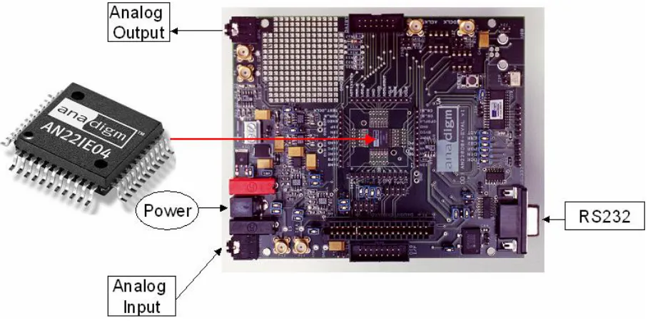
Figure 2.5. AN221E04 FPAA Chip and Evaluation Board ... 10

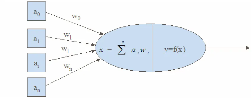
Figure 2.6. Artificial neuron model ... 13

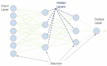
Figure 2.7. Example of feed forward neural network. ... 14

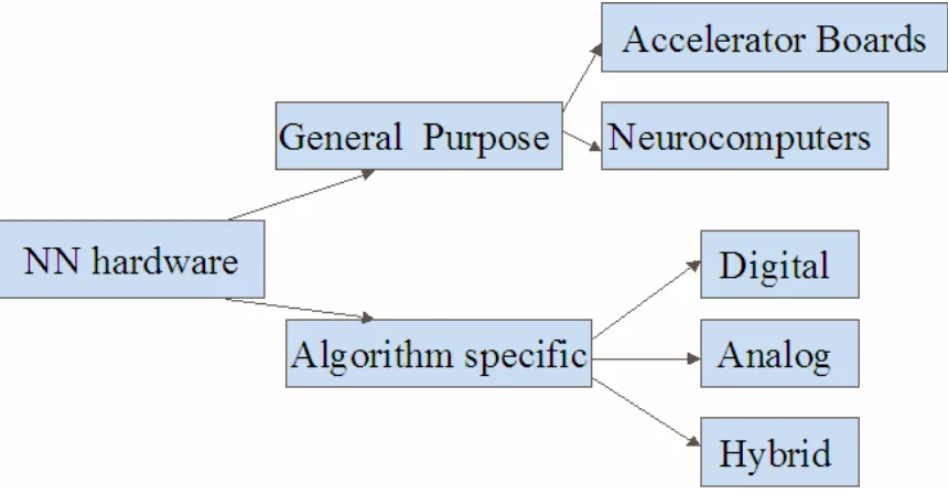
Figure 2.8. Classification of neural network hardware ... 16

Figure 2.9. FPAA circuit that implements the hyperbolic tangent function using look up table. ... 19

Figure 2.10. Look up table for the hyperbolic tangent transfer function. ... 20

Figure 3.1. The unit sigmoid function... 32

Figure 3.2. Example of data points ... 32

Figure 3.3: u₀(x) 1 tanh(ax) a = and the corresponding straight line showing the error at ) (x_N -y₁ as 4Hd ... 33

Figure 3.4. Three hyperbolic tangent functions classifying five data points ... 34

Figure 3.5. Data mapping of the two spirals problem... 37

Figure 3.7. Testing results of two-spirals problem trained with the 3-layered feed forward neural networks. (Simulated in MATLAB/SIMULINK from the MathWorks,

Natick, MA, USA)... 40

Figure 4.1. The piecewise linear (PL) activation function for _wT ₌[1,1] in two dimensions. ... 51

Figure 4.2. Obtaining the PL function using two gain stages... 53

Figure 4.3. Neural network architecture with unmerged gain blocks. ... 54

Figure 4.4. Neural network architecture with merged gain blocks... 54

Figure 4.5. Simplifying the FPAA circuit by merging G1 into the inverting sum amplifier. ... 55

Figure 4.6. XNOR-gate FPAA circuit (left) and XOR-gate FPAA circuit (right) ... 58

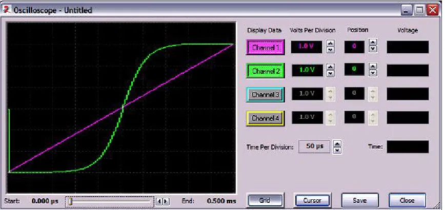
Figure 4.7. Simulation results of XNOR (channel 2) and XOR gate (Channel 4). Channel 1 and 3 are two inputs... 59

Figure 4.8. AND-gate FPAA circuit (left) and OR-gate FPAA circuit (right)... 59

Figure 4.9. Simulation results of AND (channel 2) and OR gate (Channel 4). Channel 1 and 3 are two inputs... 60

Figure 4.10. Seven decision boundaries separating 8 data points of 2 classes... 61

Figure 4.11. The output of the trained neural network view in x-z plane at y=1. ... 62

(Simulated in MATLAB/SIMULINK from the MathWorks, Natick, MA, USA) ... 62

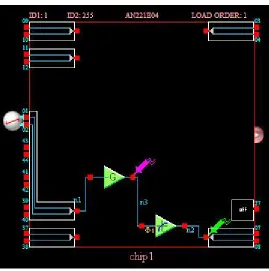
Figure 4.12. Constructing a 2-5-1 neural network using configurable analog modules of the FPAA. ... 63

Figure 4.14. The simulation results of neural network classifying two classes of data.... 65

Figure 4.15. Experimental results of neural network classifying two classes of data. ... 65

Figure 4.16. The five FPAA evaluation boards for the experiment... 66

Figure 4.17. Neural network execution time by software versus number of hidden nodes. ... 68

Figure 5.1. UGV and the path to track. Total length of the path is 380.92cm ... 77

Figure 5.2. UGV used in ADAC lab at North Carolina State University. ... 78

Figure 5.3. Birdseye view of the UGV... 79

Figure 5.4. System architecture of the FPAA - controlled unmanned ground vehicle. .... 80

Figure 5.5. The AN10DS40 Evaluation and Development System... 80

Figure 5.6. Internal circuit of photomicrosensors manufactured by OMRON... 81

Figure 5.7. The H-Bridge circuit (L293D) and its function table for each driver. ... 82

Figure 5.8. Connection between the H-bridge circuit (L293D) and DC motors. ... 83

Figure 5.9. Track for the unmanned ground vehicle testing... 84

Figure 5.10. The unmanned ground vehicle with 5 optical sensors mounted at its front end. ... 84

Figure 5.11. Sensor S1 and S5 are in asymmetrical positions of the track. ... 86

Figure 5.12. The closed-loop control of the system... 86

Figure 5.13. H-bridge circuits acts as the interface between the FPAA and the DC motors ... 88

Figure 5.14. Simulation result showing the generated PWM signal... 89

Figure 5.16. System architecture of microcontroller - controlled unmanned ground

vehicle... 90

Figure 6.1. Block diagram of the conventional PID controller. ... 100

Figure 6.2. Artificial neural network with 3 layers... 101

Figure 6.3. Example of an ANN controller in a closed-loop control... 102

Figure 6.4. Activation function of the hidden node in the ANN. ... 103

Figure 6.5. Variation of nonlinear gain k with respect to the error ... 103

Figure 6.6. Closed-loop control with disturbance... 106

Figure 6.7. Disturbance rejection performance of the PI controller and the ANN controller... 107

Figure 6.8. Step response comparison of ANN and PI controllers without disturbances. ... 108

Figure 6.9. Step response comparison of ANN and PI controllers with small disturbances. ... 109

Figure 6.10. Step response comparison of ANN and PI controllers with moderate disturbances... 109

Figure 6.11. Step response comparison of ANN and PI controllers with large disturbances. ... 110

Figure 6.12. Gaussian white noise with different noise variances... 111

Figure 6.13. Variations of gain k with different parameters. ... 112

Figure 6.14. Analysis of controllers’ sensitivity to noise... 112

Figure 6.15. UGV used in ADAC lab at North Carolina State University. ... 114

CHAPTER I - Introduction

Artificial neural networks (ANNs) play an increasingly important role in areas such as robotics [1], process control [2-3], and motor fault detection [4-6]. Both software and hardware based approaches have been used for implementing ANNs. In general, software instructions executed serially cannot take advantage of the inherent parallelism of ANN architectures. Hardware implementations of neural networks promise higher speed operation when they can exploit this massive parallelism. Different hardware implements of neural network have been reported [7-25]. Other than the FPGA based approaches [10, 11, 18, 24], most hardware implementations provide no programmability even though real-time reconfigurability of the topology or the size of an ANN could presumably improve its performance in applications where its immediate environment changes or its immediate objective is updated.

vehicle (UGV), the FPAA easily outperformed comparable digital hardware by processing the signal 8,000 times faster. Few Anadigm FPAA applications have been reported, except a voltage-to-frequency converter and a Hodgkin-Huxley neuron simulator [27-28].

Hardware requirements are important for economical implementations. Realization of ANN structures with minimal hardware is facilitated by an understanding of the general limits on the complexity required by an ANN structure for it to learn a set of examples of a certain size. This maximum complexity can be expressed as an upper bound on the neural network size. Designs of this size are guaranteed to be large enough for correct operation. Smaller ANNs might possibly operate correctly depending on the details of the problem, but any larger ANN are now guaranteed a-priori to waste neurons regardless of any particulars of the problem.

Following the introductory part of the dissertation, a literature survey of neural network hardware and the introduction to the FPAA technology is presented in Chapter II. Implementation examples of simple ANN structures are also present in the same chapter. Chapter III presents an upper bound on the complexity of feed forward neural networks - a single-hidden-layer network with at most (N/2)+1 hidden neurons is sufficient to classify N (N is even) data points of 2 classes with zero error. The upper bound reduces to (N-1)/2+1 when N is odd. The theory is then applied to design and train a neural classifier for the two-spiral problem, a benchmark problem in the neural network literature. Chapter IV applies the theory to solve another classification task and implements the ANN in the FPAA. A further neural network structure simplification technique for FPAA based ANNs is also proposed in Chapter IV. In Chapter V, an FPAA based PID controller is designed to control a path tracking unmanned ground vehicle for future performance comparison with FPAA based ANN controller. At last in Chapter VI, to demonstrate the application of FPAA based ANN in control systems, an ANN is designed in FPAA to control a path tracking unmanned ground vehicle. The performance of the FPAA based ANN controller is characterized in terms of speed, stability and robustness.

References

[1] F. L.Lewis, “Neural-network control of robot manipulators,” IEEE Expert, pp. 64-75, June 1996. [2] J. Teeter and M.-Y. Chow, “Application of Functional Link Neural Network to HVAC Thermal

[3] M.-Y. Chow and J. Teeter, “A Knowledge-Based Approach for Improved Neural Network Control of a Servomotor System with Nonlinear Friction Characteristics,” Mechatronics, vol. 5, no. 8, pp. 949-962, 1995.

[4] B. Ayhan, M.-Y. Chow, and M.-H. Song, “Monolith and Partition Schemes with LDA and Neural Networks as Detector Units for Induction Motor Broken Rotor Bar Fault Detection,” KIEE International Transactions on Electrical Machinery and Energy Conversion Systems, June 1, 2005 (invited).

[5] M.Y. Chow, “Methodologies of Using Artificial Neural Network and Fuzzy Logic Technologies for Motor Incipient Fault Detection,” World Scientific Publishing Co. Pte. Ltd., 1998.

[6] M.-Y. Chow, G. Bilbro, and S. O. Yee, “Application of Learning Theory to a Single Phase Induction Motor Incipient Fault Detection Artificial Neural Network,” International Journal of Neural Systems, vol. 2, no. 1&2, pp. 91-100, 1991.

[7] M. Holler, S. Tam, H. Castro and R. Benson, “An electrically trainable artificial neural network (ETANN) with 10240 `floating gate' synapses ,” Neural Networks, 1989. IJCNN, International Joint Conference on, pp. 191 - 196 vol.2, 18-22 June 1989.

[8] S. Tam, B. Gupta, H. Castro and M. Holler, “Learning on an Analog VLSI Neural Network Chip,” Proceedings of the IEEE International Conference on Systems, Man & Cybernetics, 1990.

[9] Y. Maeda, H. Hirano and Y. Kanata, “AN Analog Neural Network Circuit with a Learning Rule via Simutaneous Perturbation,” Proceedings of the IJCNN-93-Nagoya, pp. 853-856, 1993.

[10] S. S. Kim [1] and S. Jung, "Hardware implementation of a real time neural network controller with a DSP and an FPGA," presented at Robotics and Automation, 2004. Proceedings. ICRA '04. 2004 IEEE International Conference on, 2004.

[11] S. S. Kim W. Qinruo, Y. Bo, X. Yun, and L. Bingru, "The hardware structure design of perceptron with FPGA implementation," presented at Systems, Man and Cybernetics, 2003. IEEE International Conference on, 2003.

[13] H. Withagen, “Implementing Backpropagation with Analog Hardware,” Proceedings of the IEEE ICNN-94-Orlando Florida, pp. 2015-2017, 1994.

[14] T. Szabo, L. Antoni, G. Horvath, and B. Feher, "A full-parallel digital implementation for pre-trained NNs," presented at Neural Networks, 2000. IJCNN 2000, Proceedings of the IEEE-INNS-ENNS International Joint Conference on, 2000.

[15] S. Popescu, "Hardware implementation of fast neural networks using CPLD," presented at Neural Network Applications in Electrical Engineering, Proceedings of the 5th Seminar on, 2000.

[16] B. Girau, "Digital hardware implementation of 2D compatible neural networks," presented at Neural Networks, Proceedings of the IEEE-INNS-ENNS International Joint Conference on, 2000.

[17] H. Abdelbaki, E. Gelenbe, and S. E. EL-Khamy, "Analog hardware implementation of the random neural network model," presented at Neural Networks, Proceedings of the IEEE-INNS-ENNS International Joint Conference on, 2000.

[18] J. Zhu, G. J. Milne, and B. K. Gunther, "Towards an FPGA based reconfigurable computing environment for neural network implementations," presented at Artificial Neural Networks, Ninth International Conference on, 1999.

[19] J. Liu and M. Brooke, "A fully parallel learning neural network chip for real-time control," presented at Neural Networks, International Joint Conference on, 1999.

[20] J. Liu and M. Brooke, "Fully parallel on-chip learning hardware neural network for real-time control," presented at Circuits and Systems, Proceedings of the IEEE International Symposium on, 1999. [21] E. J. Brauer, J. J. Abbas, B. Callaway, J. Colvin, and J. Farris, "Hardware implementation of a neural

network pattern shaper algorithm," presented at Neural Networks, International Joint Conference on, 1999.

[22] P. M. Engel and R. F. Molz, "A new proposal for implementation of competitive neural networks in analog hardware," presented at Neural Networks, Proceedings. 5th Brazilian Symposium on, 1998. [23] J. Tang, M. R. Varley, and M. S. Peak, "Hardware implementations of multi-layer feed forward neural

[24] D. S. Reay, T. C. Green, and B. W. Williams, "Field programmable gate array implementation of a neural network accelerator," presented at Hardware Implementation of Neural Networks and Fuzzy Logic, IEE Colloquium on, 1994.

[25] A. Achyuthan and M. I. Elmasry, "Mixed analog/digital hardware synthesis of artificial neural

networks," Computer-Aided Design of Integrated Circuits and Systems, IEEE Transactions on, vol. 13, pp. 1073-1087, 1994.

[26] P. Dong, G. Bilbro, and M.-Y. Chow, “Controlling a Path-tracking Unmanned Ground Vehicle with a Field-Programmable Analog Array,” IEEE/ASME International Conference on Advanced Intelligent Mechatronics, Monterey, CA, 24-28 July, 2005.

[27] P. I. Yakimov, E. D. Manolov, and M. H. Hristov, "Design and implementation of a V-f converter using FPAA," presented at Electronics Technology: Meeting the Challenges of Electronics Technology Progress, 2004. 27th International Spring Seminar on, 2004.

CHAPTER II - Introduction to Field

Programmable Analog Arrays and Survey

of Artificial Neural Network Hardware

This chapter introduces FPAA technologies for ANN applications and surveys the literature of artificial neural network (ANN) hardware. Some ANN implementation examples using FPAAs are also presented.

I. The FPAA Technology

The field programmable analog array technology, which is the analog counterpart of the FPGA, appeared in 1980’s [1-8]. The technology was made commercially available by AnadigmTM in 2000. Anadigm’s FPAA chips are mainly used as platforms for experiments along with our research.

The FPAA is an array of identical Configurable Analog Blocks (CABs). Which includes operational amplifiers, comparators and switched programmable capacitors . The FPAA allows designers to implement an extremely wide variety of signal processing functions using digital configuration data.

defined for switched capacitors; its value depends on the capacitance but changes according to the sampling frequency.

Figure 2.1. Switched capacitor and its sampling clocks

As shown in Figure 2.1, capacitor C is a switched capacitor; non-overlapping clocks control two switches respectively. V_in is sampled at the falling edge of f₁, the sampling frequency is f_s . The charges going from V_in to V_out each sampling period is

) (V_in V_out C

Q= - . So the current flowing from V_in to V_out is I = f_sC(V_in -V_out). Then we

can get the equivalent resistor of resistance

C f R

s

1

= . The following two examples show

that how the switched capacitor could take the place of the resistor in an inverting integrator and a non-inverting integrator.

Figure 2.2. A normal inverting integrator

Figure 2.3. An inverting integrator with the resistor replaced by a switched capacitor

The advantage of the switched capacitors is that these are easy to build in an integrated circuit (IC) technology. It is difficult to make precise large-value resistors on silicon, but easier to make precise (and well-matched) small-value capacitors. When the switching noise is eliminated by filtering, a simple use of switched capacitor is as a resistor. For example, an effective resistance of 100 kilohms can be obtained at a switching frequency of 1 MHz by a capacitor with a capacitance of 10 pF. Switched-capacitor technology is key to the accuracy and flexibility of FPAA.

Figure 2.4. AN10E40 FPAA Chip and Evaluation Board

Figure 2.5. AN221E04 FPAA Chip and Evaluation Board

II. Introduction to Artificial Neural Networks

originated from the LVQ (Learning Vector Quantization) network underlying the idea of which was also Kohonen's in 1972 [17].

A. Application Areas of ANNs

Neural networks have been successfully applied to various data-intensive applications in industry, business and science [18]. Those applications include bankruptcy prediction [19-24], handwriting recognition [25-29], speech recognition [30], product inspection [31-32], fault detection [33-34], medical diagnosis [35-37], and bond rating [38-40]. A number of performance comparisons between neural and conventional classifiers have been made by many studies [41-43]. In addition, several computer experimental evaluations of neural networks for classification problems have been conducted under a variety of conditions [44-45].

One example of application to motor fault detection was proposed by Li, Chow, Tipsuwan and Hung [46]. They present an approach for motor rolling bearing fault diagnosis using neural networks and time/frequency-domain bearing vibration domain analysis. The results of motor bearing faults can be effectively diagnosed using neural network if the signal of motor bearing vibration is appropriately measured and translated.

B. Artificial Neuron Model and Neural Network Structures

activation function. The activation function could be linear function, step function,

sigmoid function _x

e x

f

-+ =

1 1 )

( , hyperbolic tangent function _x

x

e e x

f ₂

2

1 1 )

(

-+

-= and radial

basis function _f(_x)_=e-x2_.

Figure 2.6. Artificial neuron model

Figure 2.7. Example of feed forward neural network.

C. Overview of ANN Hardware Implementation

multiple inputs implementing neural networks has a speed advantage over software since it can take the advantage of the inherent parallelism of the ANN.

In the literature treating the hardware, implementation of neural networks, specifications include the technology used (analog, digital, or hybrid), the precision (in equivalent numbers of bits) of the input/outputs, of the weights, and of the accumulators, etc. There are two traditional criteria for the performance of neural network hardware: the first one is the MCPS or Millions of Connections Per Second, which is defined as the rate of multiply and/or accumulate operations. The other one is MCUPS or Millions of Connection Update Per Second value that denotes the rate of weight changes during network learning.

Efforts have been made to develop a more detailed classification of the neural network hardware from aspects such as system architecture, degree of parallelism or whether general-purpose or special-purpose devices are employed [48].

Figure 2.8. Classification of neural network hardware

Accelerator boards are a kind of hardware that can work in conjunction with PC to speed up the neural network implementations. They normally reside in the expansion slot. Accelerator boards are usually based on neural network chips but some just use fast digital signal processors that do multiple-accumulate operations. One example of the accelerator boards is the IBM ZISC ISA and PCI cards [49]. The ZISC is a digital chip with 64 8-bit inputs and 36 radial basis function neurons. Multiple chips can be cascaded together to create networks of arbitrary size. The ISA card holds up to 16 ZISCX036 chips providing 576 neurons and the PCI cards can hold up to 19 chips providing 684 neurons. Other accelerator cards include SAIC SIGMA-1 [50], Neuro Turbo [51] and HNC [52].

different neural networks. Neurocomputers are complex and expensive. Examples include BSP400 [53], COKOS [54] and RAP (Ring Array Processor) [55]. RAP was developed at the ICSI (International Computer Science Institute, Berkeley, CA) and has been used as an essential component in the development of connectionist algorithms for speech recognition since 1990. Implementations consist of 4 to 40 Texas Instruments TITMS320C30 floating point DSPs containing 256 Kbytes of fast static RAM and 4 Mbytes of dynamic RAM each. These chips are connected via a ring of FPGAs, each implementing a simple two-register data pipeline. Additionally each board has a VME bus interface logic, which allows it to connect to a host computer.

The algorithm specific neural network hardware (neural network VLSI) can be divided into three broad categories: digital, analog, and hybrids.

Compared to digital neural network hardware, analog hardware networks have the advantages of high speed since there is no A/D and D/A conversion needed. The first commercially available analog neural network chip is Intel’s analog ETANN chip [63]. Later more analog chips appeared such as [64-65]. Besides the advantages of high speed and high densities, since analog hardware interact directly with the real world and process signals totally in analog domain which is very fast, it is more suitable for real-time applications such as controlling unmanned vehicles compared to digital hardware.

The following section presents a new platform for ANN implementation: field programmable analog arrays (FPAAs), which can be classified into either algorithm specific or general-purpose hardware category, which are mentioned above.

III. Sample Design of ANN Using FPAA

We can conclude from the above survey that to obtain high speed and flexible neural network simulator, programmable analog hardware is desired. This paper proposes the new neural network hardware to be built using FPAA technology, which could be either algorithm specific slice analog chip or large-scale neurocomputer after integrate multiple FPAAs together.

the neural network can be arbitrarily tabulated in a look up table in each FPAA chip. Figure 2.9 is an example circuit implementing a hyperbolic tangent transfer function. The look up table as shown in Figure 2.10 was loaded from an Excel file. Figure 2.11 is the simulation result.

Figure 2.10. Look up table for the hyperbolic tangent transfer function.

IV. References

[1] D. Anderson, C. Marcjan, D. Bersch, H. Anderson, P. Hu, O. Palusinki, D. Gettman, I. Macbeth, A. Bratt, “A Field Programmable Analog Array and its Application,” 1997 Custom Integrated Circuits Conference Proceedings, May, 5-8, 1997, Santa Clara, California, USA.

[2] E.K.F. Lee and W.L. Hui, "A novel switched-capacitor based field-programmable analog array architecture," Kluwer Analog Integrated Circuits and Signal Processing - Special Issue on Field Programmable Analog Arrays, Vol. 17, No. 1-2, pp. 35-50, September 1998.

[3] S.H.K. Embabi, X. Quan, N. Oki, A. Manjrekar, and E. Sanchez-Sinencio, "A current-mode based field-programmable analog array for signal processing applications," Kluwer Analog Integrated Circuits and Signal Processing - Special Issue on Field Programmable Analog Arrays, Vol. 17, No. 1-2, pp. 125-142, September 1998.

[4] E. Pierzchala and M.A. Perkowski, "A high-frequency field-programmable analog array (FPAA) part I: design," Kluwer Analog Integrated Circuits and Signal Processing - Special Issue on Field Programmable Analog Arrays, Vol. 17, No. 1-2, pp. 143-156, September 1998.

[5] E. Lee and G. Gulak, "A CMOS field-programmable analog array," IEEE Journal of Solid-State Circuits, Vol. 26, No. 12, pp. 1860-1867, December 1991.

[6] S.T. Chang, B.R. Hayes-Gill, and C.J. Paul, "Multi-function Block for a Switched Current Field Programmable Analog Array", 1996 Midwest Symposium on Circuits and Systems, August 1996. [7] K.F.E. Lee and P.G. Gulak, "A Transconductor-Based Field-Programmable Analog Array", ISSCC

Digest of Technical Papers, pages 198-199, Feb. 1995.

[8] K.F.E. Lee and P.G. Gulak, "A CMOS Field-Programmable Analog Array", ISSCC Digest of Technical Papers, pages 186-188, Feb. 1991.

[9] McCulloch, W.S. & Pitts, W.H. “A Logical Calculus of the Ideas Immanent in Nervous Activity,” Bulletin of Mathematical Biophysics, 5: pp. 115-137, 1943.

[10] Rosenblatt, F. “The Perceptron: A Probabilistic Model for Information Storage and Organization in the Brain,” Psychological Review, 65: pp. 386-408, 1958.

[12] B. Widrow and M.E. Hoff, “Adaptive Switching Circuits,” IRE WESCON Convention Record, New York: IRE pp. 96-104, 1960.

[13] K. Fukushima, “Cognitron: A Self-organizing Multilayered Neural Network,” Biological Cybernetics, 20: pp. 121-136, 1975.

[14] D.B. Parker, “A Comparison of Algorithms for Neuron-Like Cells,” In J.S. Denker (Ed.), Neural Networks for Computing, New York: American Institute of Physics, pp. 327-332, 1986.

[15] D.D. Rumelhart, G.E. Hinton and R.J. Williams, Ronald J. “Learning Representations by Back-Propagating Errors,” Nature 323: pp. 533-536, 1986.

[16] J.J. Hopfield, “Neural Networks and Physical Systems with Emergent Collective Computational Abilities,” Proceedings of the National Academy of Sciences, 79: pp. 2554-2558, 1982.

[17] T. Kohonen, “Correlation Matrix Memories,” IEEE Transaction on Computers, C-21: pp. 353-359, 1972.

[18] B. Widrow, D. E. Rumelhard, and M. A. Lehr, “Neural networks: Applications in industry, business and science,” Communications. ACM, vol. 37, pp. 93–105, 1994.

[19] E. I. Altman, G. Marco, and F. Varetto, “Corporate distress diagnosis: Comparisons using linear discriminant analysis and neural networks (theItalian experience),” Jouranl of Bank and Finance, vol. 18, pp. 505–529, 1994.

[20] R. C. Lacher, P. K. Coats, S. C. Sharma, and L. F. Fant, “A neural net-work for classifying the financial health of a firm,” European Journal of Operations Research., vol. 85, pp. 53–65, 1995. [21] M. Leshno and Y. Spector, “Neural network prediction analysis: Thebankruptcy case,” Journal of

Neurocomputing, vol. 10, pp. 125–147, 1996.

[22] K. Y. Tam and M. Y. Kiang, “Managerial application of neural networks:The case of bank failure predictions,” Management Science., vol. 38, no. 7, pp. 926–947, 1992.

[23] R. L. Wilson and R. Sharda, “Bankruptcy prediction using neural net-works,” Decision Support System, vol. 11, pp. 545–557, 1994.

[25] I. Guyon, “Applications of neural networks to character recognition,” International Journal of Pattern Recognition and Artificial Intelligence, vol. 5, pp. 353–382, 1991.

[26] S. Knerr, L. Personnaz, and G. Dreyfus, “Handwritten digit recognition by neural networks with single-layer training,” IEEE Transactions on Neural Networks, vol. 3, pp. 962–968, 1992. [27] Y. Le Cun, B. Boser, J. S. Denker, D. Henderson, R. E. Howard, W. Hubberd, and L. D. Jackel,

“Handwritten digit recognition with a back-propagation network,” Advanced Neural Information Processing System, vol. 2, pp. 396–404, 1990.

[28] D. S. Lee, S. N. Sriharia, and R. Gaborski, “Bayesian and neural-net-work pattern recognition: A theoretical connection and empirical results with handwritten characters,” in Artificial Neural Networks and Statistical Pattern Recognition, I. K. Sethi and A. K. Jain, Eds. New York: Elsevier, pp. 89–108, 1991.

[29] G. L. Martin and G. L. Pitman, “Recognizing hand-printed letter and digits using backpropagation learning,” Neural Computing, vol. 3, pp. 258–267, 1991.

[30] H. Bourlard and N. Morgan, “Continuous speech recognition by connectionist statistical methods,” IEEE Transactions on Neural Networks, vol. 4, pp. 893–909, 1993.

[31] J. Lampinen, S. Smolander, and M. Korhonen, “Wood surface inspection system based on generic visual features,” in Industrial Applications of Neural Networks, F. F. Soulie and P. Gallinari, Eds, Singapore: World Scientific, pp. 35–42, 1998.

[32] T. Petsche, A. Marcantonio, C. Darken, S. J. Hanson, G. M. Huhn, and I. Santoso, “An autoassociator for on-line motor monitoring,” in Industrial Applications of Neural Networks, F. F. Soulie and P. Gallinari, Eds, Singapore: World Scientific, pp. 91–97, 1998.

[33] E. B. Barlett and R. E. Uhrig, “Nuclear power plant status diagnostics using artificial neural networks,” Nuclear Technology, vol. 97, pp. 272–281, 1992.

[34] J. C. Hoskins, K. M. Kaliyur, and D. M. Himmelblau, “Incipient fault detection and diagnosis using artificial neural networks,” in International Joint Conference on Neural Networks, pp. 81–86, 1990. [35] W. G. Baxt, “Use of an artificial neural network for data analysis in clinical decision-making: The

[36] H. B. Burke, “Artificial neural networks for cancer research: Outcome prediction,” Seminars in Surgical Oncology, vol. 10, pp. 73–79, 1994.

[37] H. B. Burke, P. H. Goodman, D. B. Rosen, D. E. Henson, J. N. Wein-stein, F. E. Harrell, J. R. Marks, D. P. Winchester, and D. G. Bostwick, “Artificial neural networks improve the accuracy of cancer survival pre-diction,” Cancer, vol. 79, pp. 857–862, 1997.

[38] S. Dutta and S. Shekhar, “Bond rating: A nonconservative application of neural networks,” in Proc. IEEE International Conference on Neural Networks, vol. 2, San Diego, CA, pp. 443–450, 1988. [39] A. J. Surkan and J. C. Singleton, “Neural networks for bond rating improved by multiple hidden

layers,” in Proc. IEEE International Joint Conference on Neural Networks, vol. 2, San Diego, CA, pp. 157–162, 1990.

[40] J. Utans and J. Moody, “Selecting neural network architecture via the prediction risk: Application to corporate bond rating prediction,” in International Conference on Artificial Intelligence Applications Wall Street, pp. 35–41, 1991.

[41] S. P. Curram and J. Mingers, “Neural networks, decision tree induction and discriminant analysis: An empirical comparison,” Journal of Operational Research Society, vol. 45, no. 4, pp. 440–450, 1994. [42] W. Y. Huang and R. P. Lippmann, “Comparisons between neural net and conventional classifiers,” in

IEEE International Conference on Neural Networks, San Diego, CA, pp. 485–493, 1987. [43] D. Michie, D. J. Spiegelhalter, and C. C. Taylor, Eds., Machine Learning, Neural, and Statistical

Classification, London, U.K.: Ellis Horwood, 1994.

[44] E. Patwo, M. Y. Hu, and M. S. Hung, “Two-group classification using neural networks,” Decision Science, vol. 24, no. 4, pp. 825–845, 1993.

[45] V. Subramanian, M. S. Hung, and M. Y. Hu, “An experimental evaluation of neural networks for classification,” Computers and Operations Research., vol. 20, pp. 769–782, 1993.

[47] H. McCartor, “A Highly Parallel Digital Architecture for Neural Network Emulation,” In Delgado-Frias, J. G. and Moore, W. R. (eds.), VLSI for Artificial Intelligence and Neural Networks, Plenum Press, New York, pp 357-366, 1991.

[48] T. Schoenauer, A. Jahnke, U. Roth and H. Klar, “Digital Neurohardware: Principles and Perspectives,” Proceedings of Neuronal Networks in Applications (NN'98), Magdeburg, 1998 [49] C. S. Lindsey, Th. Lindblad, G. Sekniaidze, M. Minerskjold, S. Szekely and A. Eide, “Experience

with the IBM ZISC Neural Network Chip,” Proceedings of 3rd Int. Workshop on Software

Engineering, Artificial Intelligence, and Expert Systems, for High Energy and Nuclear Physics, Pisa, Italy, April 3-8, 1995.

[50] P.C. Treleaven, “Neurocomputers,” International Journal of Neurocomputing, 1, 4-31, 1989. [51] A. F. Arif, S. Kuno, A. Iwata and Y. Yoshita, “A Neural Network Accelerator Using Matrix Memory

with Broadcast Bus,” Proceedings of the IJCNN-93-Nagoya, pp. 3050-3053, 1993.

[52] “HNC, High-Performance Parallel Computing,” SIMD Numerical Array Processor, DataSheet, San Diego.

[53] J.N. H. Heemskerk, J. Hoekstra, J.M.J., Murre, L.H.J.K. Kemna and P.T.W. Hudson, “The BSP400: A Modular Neurocomputer,” Microprocessors and Microsystems, 18, 2, pp. 67-78, 1994.

[54] H. Speckman, P. Thole and W. Rosentiel, “COKOS: A Coprocessor for Kohonen's Selforganizing Map,” Proceedings of the ICANN-93-Amsterdam, London: Springer-Verlag, pp. 1040-1045, 1993. [55] N. Morgan, J. Beck, P. Kohn, J. Bilmes, .E Allman and J. Beer, “The Ring Array Processor: A

Multiprocessing Peripheral for Connectionist Applications,” Journal of Parallel and Distributed Computing, 14, pp. 248-259, 1992.

[56] MD1220 Data Sheet, Micro Devices, 30 Skyline Dr., Lake Mary, Fl. 32746, March 1990. [57] NLX420 Data Sheet, Neurologix, Inc., 800 Charcot Av., Suite 112, San Jose, CA, June 1992. [58] N. Mauduit, M. Duranton and J. Gobert, “Lneuro 1.0: A Piece of Hardware LEGO for Building

Neural Network Systems,” IEEE Transactions on Neural Networks, 3, pp. 414-422, May 1992. [59] A. Jahnke, U. Roth, and H. Klar, “A SIMD/Dataflow Architecture for a Neurocomputer for

[60] M. Glover and W. T. Miller, “A massively-parallel SIMD processor for neural network and machine vision applications,” Proceedings NIPS-6, ed. J.D. Cowan et al., Morgan Kaufmann Pub, pp. 843-849, 1993.

[61] H. Amin, K. M. Curtis and B. R. Hayes Gill, “Two-ring systolic array network for artificial neural networks,” Circuits, Devices and Systems, IEE Proceedings, vol. 146, iss. 5, pp. 225-230, Oct. 1999. [62] U. Ramacher, “SYNAPSE - A Neurocomputer that Synthesizes Neural Algorithms on a Parallel

Systolic Engine,” Journal of Parallel and Distributed Computing, 14, pp. 306-318, 1992.

[63] S. Tam, B. Gupta, H. Castro and M. Holler, “Learning on an Analog VLSI Neural Network Chip,” Proceedings of the IEEE International Conference on Systems, Man & Cybernetics, 1990.

[64] Y. Maeda, H. Hirano and Y. Kanata, “AN Analog Neural Network Circuit with a Learning Rule via Simutaneous Perturbation,” Proceedings of the IJCNN-93-Nagoya, pp. 853-856, 1993.

[65] H. Withagen, “Implementing Backpropagation with Analog Hardware,” Proceedings of the IEEE ICNN-94-Orlando Florida, pp. 2015-2017, 1994.

[66] Synaptics, 2860 Zanker Rd., Suite 206, San Jose, Ca. 95134, USA.

[67] M. Jabri and B. Flower, “Weight Perturbation: An Optimal Architecture and Learning Technique for Analog VLSI Feed forward and Recurrent Multi-Layer Networks,” Neural Computation, vol. 3, pp. 546-565, 1991.

[68] V. F. Koosh and R. M. Goodman, “VLSI neural network with digital weights and analog

multipliers,” Proc. IEEE International Symposium on Circuits and Systems, vol. III, pp. 233-236, May 2001.

[69] S. Churcher, D. J. Baxter, A. Hamilton, A. F. Murray and H. M. Reekie, “Generic Analog Neural Computation-the Epsilon Chip,” Advances in Neural Information Processing Systems: Proceedings of the 1992 Conference, Denver, Colorado.

[70] Y. Hirai, “A 1,000-Neuron System with One Million 7-bit Physical Interconnections,” In Jordan, M.I., Kearns, M.J. and Solla, S.A. eds. Advances in Neural Information Processing Systems 10, A

[71] B. Kim, C. Kim, S. Han, S. Kim and H. Park, “1.2-μM non-epi CMOS smart power IC with four H-bridge motor drivers for portable applications,” Circuits and Systems, ISCAS '96., 'Connecting the World'., 1996 IEEE International Symposium on , Vol.1 pp: 633 – 636, 12-15 May 1996 [72] Datasheet of L293D by Texas Instrument Inc.

[73] Product GH12-1828Y of Jameco Electronics Inc.

[74] N.N. Bengiamin and M. Jacobsen, “Pulse-width modulated drive for high performance DC motors,” Industry Applications Society Annual Meeting, 1988., Conference Record of the 1988 IEEE, Vol.1, pp:543 – 550, 2-7 Oct. 1988.

[75] www.handyboard.com

[76] M.-Y. Chow, G. Bilbro, and S. O. Yee, “Application of Learning Theory to a Single Phase Induction Motor Incipient Fault Detection Artificial Neural Network,” International Journal of Neural Systems, vol. 2, no. 1&2, pp. 91-100, 1991.

[77] J. Van der Spiegel, P. Mueller, V. Agami, P. Aziz, D. Blackman, P. Chance, A. Choudhury, C. Donham, R. Etienne-Cummings, L. Jones, J. Kim, P. Kinget, M. Massa, W. von Koch, J. Xin, “A multichip analog neural network,” Proceedings of Technical Papers, International Symposium on VLSI Technology, Systems, and Applications, pp. 64 – 68, 22-24 May 1991

[78] S. Tam, M. Holler, J. Brauch, A. Pine, A. Peterson, S. Anderson, S. Deiss,”A reconfigurable multi-chip analog neural network: recognition and back-propagation training,”International Joint Conference on Neural Networks, 1992., Vol. 2, pp. 625-630, 7-11 June 1992

[79] P. Hasler, L. Akers, “Implementation of analog neural networks,” Tenth Annual International Phoenix Conference on Computers and Communications, pp. 32-38, 27-30 March 1991 [80] M. Ponca, G. Scarbata, "Implementation of Artificial Neurons Using Programmable Hardware,"

CHAPTER III - Upper Bound on the Size

of Neural Networks for Data

Classification

1 _{Department of Electrical and Computer Engineering,} North Carolina State University, Raleigh NC 27695 USA

* Corresponding Author

This work has been submitted to IEEE Transactions on Neural Networks Puxuan Dong1

IEEE Student Member [email protected]

Griff Bilbro1* IEEE Senior Member

Abstract

This paper proposes an upper bound on the complexity of feed forward neural networks for classifying data. We show that N data points drawn from two classes can be correctly labeled by a network with a single hidden layer network containing at most N/2+1 hidden neurons (when N is even or (N-1)/2+1 hidden neurons when N is odd) with hyperbolic tangent activation functions.

Keywords: upper bound, classification, feed forward neural network

I. Introduction

Proper size of a neural network (NN) allows it to learn a task efficiently and to predict future output appropriately [1] and has been considered by several researchers. Lecun proposed optimal brain damage [2]; Hassibi presented optimal brain surgeon [3]; Mozer “trimmed” the excessive neuron and weights from the neural network via relevance assessment, which he called “Skeletonization” [4]. The initial maximum necessary network size is desired for pruning techniques since it makes the techniques efficient. Besides the pruning techniques mentioned above, there are also constructive methods such as cascade-correlation (CC) introduced by Falman [5]. Thivierge, Rivest and Shultz even found a way to prune constructive neural networks which is a “dual phase” technique [6].

capability is also important since it helps to choose the size of neural networks. Excessively large neural networks are computationally demanding to simulate and may not generalize appropriately; and on the other hand, neural networks of inadequate complexity may fail to learn significant features of a data set. A lower bound on the size of the neural network was recently reported by Gao and Ji [15].

In this paper we present an upper bound for the size of the neural network solving classification problems. We show that a conventional three-layer feed forward neural network with hyperbolic tangent activating functions containing K+1 neurons in its hidden layer can learn any arbitrary assignment of 2K vectors to two classes.

We apply the proposed theory to the two spirals benchmark problem [17]. We find that a neural network with the proposed number of hidden neurons learns the two-spiral problem perfectly within 500 training epochs. This is about 70% less training effort than for the cascade-correlation algorithm proposed by Fahlman and Lebiere [5]. We also find that networks with 15% fewer neurons than the proposed upper bound cannot learn the data without error.

The paper is organized as follows: section II derives the upper bound; section III applies the theory to a benchmark classification problem - the two-spiral problem and section IV offers some concluding remarks.

II. Theory

of the input data vectors [15]. We therefore restrict our attention to the one-dimensional case to analyze the upper bound on the number of hidden neurons of a single-hidden-layer feed forward neural network solve two-class classification problems of N data points.

In one dimension, the alternate label problem [16] requires the most decision points since when elements from different classes of data alternate with each other, each pair of adjacent points needs one decision point between them. The N-point alternate label problem needs N-1 decision points and provides an upper bound on the number of hidden neurons required for classification.

For simplicity, we choose { 1, 1}+ - as the label set for the alternate label problem. This is equivalent to using the algebraic sign of the neural network output as the label that it computes for a particular input value. This can also be described as choosing a threshold value of zero for the real-valued function computed by the neural network.

We assume that the number N =2K+1of data points is odd, that they are indexed by size so thatx₁<x₂ <x_3L<x_2K+1, that the odd points are labeled 1+ , and that the even points are labeled 1- . We define 1

(

)

1 1

1 max 2

N

n n n

H º ₌- x ₊ -x to be half the maximum

interval between adjacent data points and 1

(

)

1 min 2

N

n n n

h - x x

= +

º - to be half the minimum

(

)

1 )

(x x

u = + b shown in Figure 3.1 where b is chosen to solve

d

b ) 1 2

tanh( x = - for 4

h KH

d = so that u³ -1 dfor x h³ and u£d for x£ -h.

Figure 3.1. The unit sigmoid function

It is convenient to define a second set of N points as y_n ºx_n -hfor 1£ £k N as indicated in Figure 3.2. It follows from these definitions for appropriate n that x_n-y_n =h, and h y£ _n+1-x_n £H , and 2h x£ _n+1-x_n = y_n+1-y_n £2H .

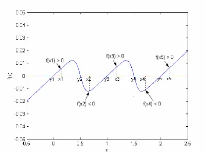
Figure 3.2. Example of data points

We define the function u x₀( ) 1 tanh(ax)

a

= to be approximately linear in the interval

x x

relationship between (x_N -y₁)and u₀(x) 1tanh(ax)

a

= is shown in Figure 3.3. It follows

that x-y₁-4Hd £u₀(x-y₁)£x-y₁.

Figure 3.3: u₀(x) 1 tanh(ax)

a

= and the corresponding straight line showing the error at (x_N - y₁)as

d

H 4

We now show that the function _{0 1}

(

) (

)

1

( ) ( ) K _{k k k}

k

f x u x y y ₊ y _- u x y =

= - -

å

Figure 3.4. Three hyperbolic tangent functions classifying five data points

In the expression _{2 0 2 1}

(

) (

)

1

( _n) ( _n ) K _{k k n k}

k

f x u x y y ₊ y _- u x y =

= - -

å

the sum into two parts. In the first part over 1£ £k n we have x_2n-y_2k ³h so that

2 2

( _{n k}) 1

u x -y ³ -d . In the second part overn+ £ £1 k Kwe have x_2n -y_2k £ -h and we assert only thatu>0 , so that _{2 2 1}

(

)

(

)

1 1

( _n) _n n _{k k} n _{k k}

k k

f x x y y ₊ y _- y ₊ y _- d

= =

£ - -

å

å

The first sum telescopes to y_2n+1-y₁ and combines with the first two terms to yield

2n 2n 1

x -y ₊ £ -h . The second term is less than 4n Hd , so that

2

( _n) 4 4

For the remaining data points, we have

(

) (

)

2 1 0 2 1 1 2 1 2 1 2 1 2 1

( _n ) ( _n ) K _{k k n k}

k

f x + u x + y y + y - u x + y =

= - -

å

sum into two parts. For n+ £ £1 k K , we have x_2n+1 -y_2k £ -h so that

2 1 2

( _{n k})

u x ₊ -y £d and we have u<1 for all k including 1£ £k n . In addition

0( 2n 1 1) 2n 1 1 4

u x ₊ -y ³ x ₊ -y - Hd by construction. Consequently we can

write _{2 1 2 1 1}

(

)

(

)

1 1

( _n ) _n 4 n _{k k} K _{k k}

k k n

f x + x + y Hd y + y - y + y - d

= = +

³ - - -

å

å

first sum telescopes as before and combines with the first two terms. The second sum is

bounded above by

1 4 K k n Hd = +

å

(

)

2 1 2 1 2 1

( _n ) _{n n} 4 4 1 4 ( )

f x ₊ ³ x ₊ -y ₊ - Hd - H K n- - d = -h H K n- d . But K n K- £ so that this implies that f x( _2n+1)³ -h 4HKd = -h h and we can conclude that f x( _2n+1) 0³ , as desired.

Therefore, 2K+1 points can be classified correctly by K+1 neurons in the hidden layer of a feed forward neural network. In other words, (N -1)/2+1hidden neurons are sufficient to classify N data points of two classes.

network. In other words, N/2+1 hidden neurons are sufficient to classify N data points of two classes.

Since f is contained in the set of functions naturally realized by conventional three-layer feed forward neural networks, we have shown that a single-hidden-three-layer network with at most (N/2)+1 hidden neurons is sufficient to classify N (N is even) data points of 2 classes with zero error. The upper bound reduces to (N-1)/2+1 when N is odd. Since this problem is the worst case of any one-dimensional problem of size Nand since the number of hidden layer neurons does not depend on the dimension of the inputs, we have shown that any 2-labeling problem of size N can be learned without error by a conventional feed forward neural network with at most N/ 2 1+ hidden neurons.

III. Experimental Results

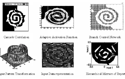
Figure 3.5. Data mapping of the two spirals problem.

the computational complexity and branch control network add additional structure to the existing neural network which adds complexity to training as well.

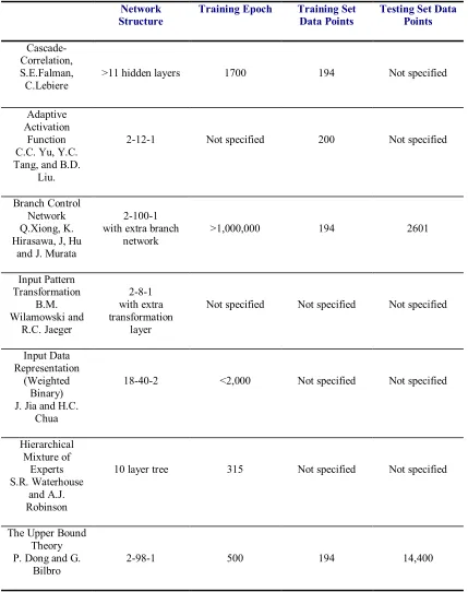
Table 3.1. Comparison of different methods classifying the two-spiral problem.

Network

Structure Training Epoch Training Set Data Points Testing Set Data Points

Cascade-Correlation, S.E.Falman, C.Lebiere

>11 hidden layers 1700 194 Not specified

Adaptive Activation

Function C.C. Yu, Y.C. Tang, and B.D.

Liu.

2-12-1 Not specified 200 Not specified

Branch Control Network Q.Xiong, K. Hirasawa, J, Hu

and J. Murata

2-100-1 with extra branch

network >1,000,000 194 2601

Input Pattern Transformation B.M. Wilamowski and R.C. Jaeger 2-8-1 with extra transformation layer

Not specified Not specified Not specified

Input Data Representation

(Weighted Binary) J. Jia and H.C.

Chua

18-40-2 <2,000 Not specified Not specified

Hierarchical Mixture of Experts S.R. Waterhouse and A.J. Robinson

10 layer tree 315 Not specified Not specified

The Upper Bound Theory P. Dong and G.

Figure 3.6. Generalization performance of two-spiral problem by different methods.

3.7(a) 40 hidden neurons _{3.7(b) 40 hidden neurons}

3.7(c) 60 hidden neurons _{3.7(d) 60 hidden neurons}

3.7(e) 70 hidden neurons 3.7(f) 70 hidden neurons

3.7(g) 80 hidden neurons 3.7(h) 80 hidden neurons

3.7(i) 90 hidden neurons 3.7(j) 90 hidden neurons

3.7(k) 98 hidden neurons _{3.7(l) 98 hidden neurons}

3.7(m) 145 hidden neurons 3.7(n) 145 hidden neurons

As shown in Figure 3.7, the testing results indicate the network classifies the problem better with the increase of the number of the hidden neurons. The network classifies the two groups of data completely when the neuron number reaches 90 in the hidden layer. With 98 and 145 neurons in the hidden layer, the network still classifies the two groups of data points successfully. This means the minimum required neuron numbers is between 80 - 90 which is fairly close to our calculated “data-independent” upper bound. This result would be closer to our upper bound if the problem could somehow be made more difficult.

For the 2-98-1 structure, the classification error on the training set of 194 points drops to zero after 500 back propagation training epochs. The trained network classifies the two groups of data with 100 percent accuracy. The number of epochs is 70.59% less than the result (1700 epochs) obtained by the cascade-correlation algorithm proposed by Fahlman and Lebiere [5].

IV. Conclusion

An upper bound has been presented for the number of neurons in the hidden layer of a 3-layered neural network that can correctly label any N data points of 2 classes. At most N/2+1 hidden neurons is sufficient to classify N such data points of 2 classes with zero error. The hidden neurons have hyperbolic tangent activation functions. The data points are allowed to be m dimensional (m > 1). The application of the theory is demonstrated with a classification benchmark problem from the literature.

V. References

[1] Z. Qin and Z. Mao, "A new algorithm for neural network architecture study," presented at Intelligent Control and Automation, 2000. Proceedings of the 3rd World Congress on, 2000. [2] Y. LeCun, J. Denker & S. Solla, “Optimal Brain Damage,” In D. Touretzky (ed.), Advances in

Neural Information Processing Systems, Morgan Kaufmann, pp. 598-605. San Mateo, CA, 1990. [3] B. Hassibi, D. G. Stork, “Second order derivatives for network pruning: Optimal Brain Surgeon,”

Proceedings of Neural Information Processing Systems, pp.164-171, 1993.

[4] M. C. Mozer & P. Smolensky, “Skeletonization: A technique for trimming the fat from a network via relevance assessment,” Advances in Neural Information Processing Systems, pp. 107-115, 1998.

[5] S. E. Fahlman and C. Lebiere, “The cascade-correlation learning architecture,” In Touretzky, D. S., editor, Advances in Neural Information Processing Systems, pp. 524-532, San Mateo, 1990. [6] J. P. Thivierge, F. Rivest, T.R. Shultz, “A dual-phase technique for pruning constructive networks,”

Proceedings of the IEEE International Joint Conference on Neural Networks, pp. 559-564, 2003. [7] E. Baum, “On the capabilities of multilayer perceptrons,” Journal of Complexity, vol. 4, pp. 193–

215, 1988.

[9] I. Ciuca, "On the approximation capability of neural networks using bell-shaped and sigmoidal functions," presented at IEEE International Conference on Systems, Man, and Cybernetics, 1998. [10] W. Eppler and H. N. Beck, "Piecewise linear networks (PLN) for function approximation,"

presented at Neural Networks, 1999. IJCNN '99. International Joint Conference on, 1999.

[11] Z. Zhanga, X. Mab and Y. Yang, “Bounds on the number of hidden neurons in three-layer binary neural networks,” Neural Networks 16, 2003.

[12] K. H. Schindler, M. Sanguineti, “Bounds on the complexity of neural-network models and comparison with linear methods,” International Journal of Adaptive Control and Signal Processing. Vol, 17, pp. 179-194, 2003.

[13] G. B. Huang, “Learning Capability and Storage Capacity of Two-Hidden-Layer Feed forward Networks,” IEEE Transactions on Neural Networks, vol. 14, no. 2, Mar. 2003.

[14] G. B. Huang and H. A. Babri, "Upper Bounds on the Number of Hidden Neurons in Feed forward Networks with Arbitrary Bounded Nonlinear Activation Functions," IEEE Transactions on Neural Networks, vol. 9, no. 1, pp. 224-229, 1998.

[15] D. Gao and Y. Ji, “Classification methodologies of multilayer perceptrons with sigmoid activation functions, ” Pattern Recognition 38 pp. 1469 – 1482, 2005

[16] S. Ridella, S. Rovetta, and R. Zunino, "Circular back propagation networks for classification," IEEE Transactions on Neural Networks, vol. 8, pp. 84-97, 1997.

[17] K. K. Lang and M. K. Witbrock, “Learning to tell two spirals apart,” in Proceedings of Connectionist Models Summer School, San Mateo, CA: Morgan Kaufman, pp. 52-61, 1998. [18] J. Jia and H. C. Chua, “Solving two-spiral problem through input data representation,” Neural

Networks, 1995. Proceedings., IEEE International Conference on, vol. 1, pp. 132 – 135, 27th Nov.-1st Dec. 1995.

[19] S. Ridella, S. Rovetta and R. Zunino, “Representation and generalization properties of class-entropy networks,” IEEE Transactions on Neural Networks, vol. 10, issue 1, pp. 31-47, Jan 1999. [20] H. C. Fu, Y. L. Lee, C. C. Chiang and H. T. Pao, “Divide-and-conquer learning and modular

[21] C.-C. Yu, Y.-C. Tang, and B.-D. Liu, "An adaptive activation function for multilayer feed forward neural networks," presented at TENCON '02. Proceedings. 2002 IEEE Region 10 Conference on Computers, Communications, Control and Power Engineering, 2002.

[22] Q. Xiong, K. Hirasawa, J. Hu, and J. Murata, "Comparative study between functions distributed network and ordinary neural network," presented at Systems, Man, and Cybernetics, 2001 IEEE International Conference on, 2001.

[23] B. M. Wilamowski and R. C. Jaeger, "Implementation of RBF type networks by MLP networks," presented at Neural Networks, 1996., IEEE International Conference on, 1996.

[24] S. R. Waterhouse and A. J. Robinson, "Classification using hierarchical mixtures of experts," presented at Neural Networks for Signal Processing [1994] IV. Proceedings of the 1994 IEEE

CHAPTER IV -

Implementation of

Artificial Neural Network for Real Time

Applications Using Field Programmable

Analog Arrays

¹ Advanced Diagnosis Automation & Control Lab, Department of Electrical and Computer Engineering, North Carolina State University, Raleigh NC 27695 USA

Phone: +1(919)515-5405

² Department of Electrical and Computer Engineering, North Carolina State University, Raleigh NC 27695 USA

* Corresponding Author

This chapter is to be submitted to IEEE Transactions on Computational Intelligence. A short version of this work is accepted for presentation in WCCI2006 (International Joint

Conference on Neural Netwoks, Vancouver, BC, Canada, July 16-21). Puxuan Dong1*

IEEE Student Member [email protected]

Mo-Yuen Chow1 IEEE Senior Member

[email protected] Griff Bilbro2

Abstract

This paper presents a method of realizing artificial neural networks (ANNs) hardware implementation using field programmable analog arrays (FPAAs). A simplified realization for neurons with piecewise linear activation functions is used to reduce the complexity of the neural network architecture. Several different feedforward neural networks are implemented using single-chip and multi-chip FPAAs. Anadigm’s commercially available AN221E04 FPAA chips are adopted as the platform for simulation and experiments. The FPAA based multi-chip ANN classifies two groups of data with zero error at a speed of 6.0 Million Connections Per Second (MCPS). The result is more than 1400 times faster than comparable software implementation. The ANN architecture is also expandable to perform more complicated tasks by incorporating more FPAA chips into the implementation. The programmability of the FPAA makes analog rapid prototyping possible.

Keywords: field programmable analog arrays, neural network hardware, rapid prototyping

I. Introduction

hardware implements of neural network have been reported [7-25]. Other than the FPGA based approaches [10, 11, 18, 24], most of the hardware implementations provide no programmability. Reconfigurability of an ANN is desirable since many ANN applications, e.g., robots performing different tasks in different environments may benefit from different neural network topologies (e.g., different number of hidden nodes). The best choices for neural network implementations that achieve both high speed and rapid prototyping appear to be programmable hardware approaches like field programmable gate arrays (FPGAs) and field programmable analog arrays (FPAAs). Compared to digital hardware, FPAAs have the advantage of interacting directly with the real world because they receive, process, and transmit signals totally in the analog domain (without the need to do A/D, D/A conversions) and are suitable for real time applications. As reported in [26] on controlling a path-tracking unmanned ground vehicle, an FPAA can easily outperform the digital hardware by processing the signal 8,000 times faster. Other FPAA applications, including a voltage-to-frequency converter and a Hodgkin-Huxley neuron simulator, have been reported [27-28].