Asynchronous Parallel Learning for Neural Networks and Structured
Models with Dense Features
Xu Sun
∗MOE Key Laboratory of Computational Linguistics, Peking University
†School of Electronics Engineering and Computer Science, Peking University
Abstract
Existing asynchronous parallel learning methods are only for the sparse feature models, and they face new challenges for the dense feature models like neural networks (e.g., LSTM, RNN). The problem for dense features is that asynchronous parallel learning brings gradient errors derived from overwrite actions. We show that gradient errors are very common and inevitable. Never-theless, our theoretical analysis shows that the learning process with gradient errors can still be convergent towards the optimum of objective functions for many practical applications. Thus, we propose a simple methodAsynGrad for asynchronous parallel learning with gradient error. Base on various dense feature models (LSTM, dense-CRF) and various NLP tasks, experiments show thatAsynGrad achieves substantial improvement on training speed, and without any loss on accuracy.
1 Introduction
Stochastic learning methods can accelerate the training speed compared with traditional batch training methods. A widely used stochastic learning method is the stochastic gradient descent method (SGD) (Bertsekas, 1999; Bottou and Bousquet, 2008; Shalev-Shwartz and Srebro, 2008; Sun et al., 2012; Sun et al., 2014). For large-scale datasets, the SGD training methods can be much faster than batch training methods. For further improve the training speed over multi-core machines and clusters, a variety of asynchronous (lock-free) parallel learning methods has been developed based on stochastic learning (Niu et al., 2011; Mcmahan and Streeter, 2014). Those asynchronous methods have shown to be more efficient than the synchronous (locked) parallel learning versions (Langford et al., 2009; Gimpel et al., 2010). Other related work on parallel stochastic learning also includes (Zinkevich et al., 2010; Dekel et al., 2012; Recht and Re, 2013; Dean et al., 2012).
Existing asynchronous parallel learning methods are mainly for the sparse feature models, and feature sparseness is a major assumption for those parallel learning methods (Niu et al., 2011; Mcmahan and Streeter, 2014). For example, Niu et al. (2011) proposed an interesting asynchronous parallel learning methodHogWildfor strict sparse machine learning problems with sparse separable cost functions (e.g., sparse SVM, low-rank matrix completion). Niu et al. (2011) stated that the key idea that underlies their lock-free approach is that the targeted machine learning problems are sparse. More recently, Mcmahan and Streeter (2014) proposed a delay-tolerant asynchronous parallel learning method, which is an ex-tension of the method of Niu et al. (2011). This asynchronous parallel learning method proposed by Mcmahan and Streeter (2014) also strictly requires the sparseness of the features.
The situation is different for the dense feature models like neural networks (e.g., LSTM, RNN). Since the existing asynchronous parallel learning methods are strictly for sparse feature models, it is no longer reasonable to apply those methods for the dense feature models like neural networks. To our knowledge, there is very limited study on developing asynchronous parallel learning methods for neural networks. In most cases only synchronous versions of parallel learning are applied to neural networks, such as
This work is licenced under a Creative Commons Attribution 4.0 International License. License details: http:// creativecommons.org/licenses/by/4.0/
R
G
W W
G
R R&G
W
W
R&G R
G
W
W G R
Thread-1
Thread-2 Thread-1
Thread-2
Thread-1
Thread-2
R-overwrite
W-overwrite
[image:2.595.123.477.62.208.2](a) Simple case (b) Grad delay case (c) Grad error case
Figure 1: Illustrations of thesimple case(left), thegradient delay case(middle), and thegradient error case(right) based on stochastic parallel learning. G means the gradient-computing action. R means the read action of shared memory. W means the write action.
GPU-based and mini-batch-based parallel learning methods. For GPU-based parallel learning, a matrix is computed in a synchronously parallelized way by using GPU units. For mini-batch-based parallel learning, the gradient of a mini-batch of samples are calculated in a synchronously parallelized way as well.
The major problem for applying asynchronous parallel learning to dense feature models is from the gradient errors. We show that gradient errors are very common and inevitable in applying asynchronous parallel learning to dense feature models. Suppose a dense feature model with 10 features/parameters, and we apply asynchronous (lock-free) parallel learning. When one thread is computing gradient, it needs to read the parameters from the shared memory. It is possible that 5 parameters are overwritten by another thread, which makes the computed gradient wrong. Not only there can be read-overwrite errors, but also there can be write-overwrite errors, as shown in Figure 1 (right).
Figure 1 illustrates the simple case (left), thegradient delay case (middle), and thegradient error case(right) for stochastic parallel learning. The simple case is normally from the synchronous parallel learning setting. The gradient delay case is considered for asynchronous parallel learning over sparse feature models (Niu et al., 2011; Mcmahan and Streeter, 2014). Essentially, the gradient delay problem is a simplification of the asynchronous parallel learning problem, and the simplification is from the feature sparseness. For the dense feature models like neural networks, it is unreasonable to use this simplification, and it goes to the gradient error case. As we can see from Figure 1 (right), there are both read-overwrite and write-overwrite problems between the two threads, and this created the gradient error. The gradient error problem is more complex than the gradient delay problem, and it requires new analysis and solutions. We will give more detailed analysis in Section 2.
Although the gradient error problem is more complex, it does not mean that the asynchronous parallel learning is doomed for the dense feature models. We give theoretical analysis to show that the learning process with the gradient error problem can still achieve the optimum given certain conditions, and those conditions are usually valid for the final convergence region of real-world applications.
Based on the analysis, we propose a simple asynchronous parallel learning method for dense feature models including neural networks and other structured models, and it works well in real-world NLP tasks in spite of gradient errors. Base on various dense feature models (LSTM, dense-CRF) and various NLP tasks, experiments show that our method achieves substantial improvement on training speed, and without any loss on accuracy.
2 AsynGrad: Asynchronous Parallel Learning with Gradient Error
Algorithm 1AsynGrad: Asynchronous Parallel Learning with Gradient Error Input: model weightswww, training setSofmsamples
Runkthreads in parallel with share memory, and procedure of each thread is as follows: repeat
Get a samplezzzuniformly at random fromS
Get the update termssszzz(www), which is computed as∇fzzz(www)but usually contains error
Updatewwwsuch thatwww←www−γssszzz(www)
untilConvergence returnwww
the gradients (Niu et al., 2011; Mcmahan and Streeter, 2014). In Figure 1 (middle), thread-1’s gradient is delayed by thread-2, because the former is expected to write to the memory before thread-2’s write action. TheHogWildmethod (Niu et al., 2011) and the delay-tolerant method (Mcmahan and Streeter, 2014) mainly cast/simplify the asynchronous parallel learning problem as the gradient delay problem, and they give solutions accordingly — they show that asynchronous parallel learning can achieve the optimum when dealing with the gradient delay problem.
The gradient delay problem is a simplification of the asynchronous parallel learning problem, and the simplification is from the feature sparseness. For the dense feature models like neural networks, it is no longer reasonable to use the simplification. The major problem for applying asynchronous parallel learning to dense feature models is the gradient errors.
As shown in Figure 1 (right), for dense feature models the read action is together with the gradient-computing action. When the feature is dense, it is not efficient to read all the parameters into a thread before computing the gradient. Also, when the feature is dense, the write action is no longer a fast action. As we can see from Figure 1 (right), there are both read-overwrite and write-overwrite problems, which create gradient errors. The gradient error problem is more complex than the gradient delay problem, and it requires new analysis and solutions.
2.1 AsynGradAlgorithm
Letf(www)be the objective function of dense feature model andwww ∈ W is the weight vector. Recall that the SGD update with learning rateγ has a form like this:
wwwt+1←wwwt−γ∇fzzzt(wwwt) (1)
wheretrepresents a time stamp, and∇fzzz(wwwt)is the stochastic estimation of the gradient based onzzz,
which is randomly drawn from the training setS.
Then, we assume a shared memory machine with multiple processors, and a vector of variableswwwin the shared memory is accessible to all processors. Each processor can read and updatewww.
Based on the multicore computing machine, the proposed method createskparallel threads, andwwwis shared among thekthreads. For each thread, it gets a samplezzz uniformly at random from the training setS. Then, it tries to compute the update termssszzz(www)as follows:
ssszzz(www)←≈∇fzzz(www) (2)
where ←≈ means thesss
zzz(www) is computed as the gradient ∇fzzz(www) in a single thread, but the shared
weightswww may be partially or completely overwritten by other threads when computing the gradient, which leads to gradient errors of∇fzzz(www). Hence,ssszzz(www) is an approximation of the gradient ∇fzzz(www)
with potential errors.
Then, the thread updates the shared weightswwwbased on the update termssszzz(www), such that
w
ww←www−γssszzz(www) (3)
To summarize, the proposed parallel learning algorithm calledAsynGradis shown in Algorithm 1. Although the implementation ofAsynGradis simple, the methodAsynGraditself is not that straight-forward, because people may think it is wrong to use a method likeAsynGrad. There is not much existing theoretical analysis and empirical evidence supporting the design ofAsynGrad. In this paper, we show that it is actually reasonable and promising to use a method likeAsynGrad. We give theoretical justifica-tion of the convergence ofAsynGradbased on certain conditions, and we show experimental results that AsynGradindeed works well in practice.
2.2 Theoretical Analysis ofAsynGrad
AlthoughAsynGraddoes the weight update in parallel from different threads, from the viewpoint ofwwwit simply receives a sequence of gradient updates (but with potential errors, which is the major difference from non-parallel SGD learning). In other words, the AsynGrad learning problem can be casted as a traditional SGD learning problem, and the only difference compared with traditional SGD is that the gradients are with errors. To state our convergence analysis results, we need several assumptions.
We assumef is strongly convex with modulusc, that is,∀www,www′ ∈ W,
f(www′)≥f(www) + (www′−www)T∇f(www) + c2||www′−www||2 (4)
where|| · ||means 2-norm|| · ||2by default in this work. For some dense feature models like dense-CRF,
this assumption is suitable for the objective function. For some other dense feature models like neural networks, this assumption is a bit too strong because we know that the objective function of neural networks is non-convex. Nevertheless, even when the objective function is non-convex, the assumption usually holds within the final convergence region because the cost function is locally convex in many practical applications.
We also assume Lipschitz continuous differentiability of∇fwith the constantq, that is,∀www,www′∈ W,
||∇f(www′)− ∇f(www)|| ≤q||www′−www|| (5)
Also, let the norm ofssszzz(www)is bounded byκ∈R+:
||ssszzz(www)|| ≤κ (6)
Moreover, it is reasonable to assume
γc <1 (7)
because even the ordinary gradient descent methods will diverge ifγc >1(Niu et al., 2011).
Based on the conditions, we show thatAsynGradconverges closely towards the minimum (optimum)
www∗off(www)with a small distance expressed byϵ, and the convergence rate is given as follows.
Theorem 1(AsynGradconvergence and convergence rate). With the conditions (4), (5), (6), (7), letϵ >0
be a target distance of convergence (i.e., the closeness of the convergence point to the real optimum). Let
τ denote the bound to describe the severeness of gradient errors, such that
[∇f(www)−sss(www)]T(www−www∗)≤τ (8)
wherewwwis the weight vector duringAsynGrad training, andsss(www) is expectedssszzz(www)overzzz such that sss(www) =Ezzz[ssszzz(www)]. Letγ be a learning rate as
γ = cϵβqκ−22τq (9)
where we can setβas any value as far asβ ≥1. Lettbe the number of updates as follows
Table 1: Some major experimental results on dense-CRF. Time means time cost per iteration. Method Acc (%) Time (s) F-score (%) Time (s) F-score (%) Time (s)POS-Tag Chunking MSR-WordSeg
SGD 97.18 466.08 94.55 1.92 97.13 64.94
AsynGrad(10-thread) 97.18 108.38 94.59 0.25 97.15 8.11
AsynGrad(10-thread)+SR 97.35 25.99 94.60 0.21 97.22 6.59
where=. means ceil-rounding of a real value to an integer, anda0 is the initial distance such thata0 =
||www0−www∗||2. Then, aftertupdates ofwww,AsynGradconverges towards the optimum such thatE[f(wwwt)− f(www∗)]≤ϵ, as far as the gradient errors are bounded such that
τ ≤ 2cϵq (11)
The proof is in Section 4.
This theorem shows thatAsynGradis also convergent towards the optimum of the objective function, as far as the gradient errors are bounded such that Eq.(11) holds. For real-world applications, those assumptions and conditions usually hold at the final convergence region. In the final convergence region,
wwwis not far away from the optimumwww∗, and both||∇f(www)||and||sss(www)||are supposed to be small. Thus,
[∇f(www)−sss(www)]T(www−www∗)is supposed to be small. This makes the boundτ to be small, which makes
Eq.(11) valid in the final convergence region.
Moreover, the convergence rate is given in the theorem —AsynGradis guaranteed to converge witht
updates, and the value oftis given by Eq.(10).
The theoretical analysis can be concluded as follows. First, it shows thatAsynGradis convergent with gradient errors by given certain assumptions and conditions. Second, those assumptions and conditions are usually valid in the final convergence region of practical applications. Third, the convergence speed is given.
3 Experiments
We conduct experiments on natural language processing tasks as follows. Experiments are performed on a computer based on Intel(R) Xeon(R) 3.0GHz CPU of 12 cores, and with 128G memory.
Part-of-Speech Tagging (POS-Tag): We use the standard benchmark dataset in prior work (Collins, 2002), which is derived from PennTreeBank corpus and uses sections 0 to 18 of the Wall Street Journal (WSJ) for training (38,219 samples), and sections 22-24 for testing (5,462 samples). The evaluation metric is per-word accuracy.
Text Chunking (Chunking): The phrase chunking data is extracted from the data of the CoNLL-2000 shallow-parsing shared task(Sang and Buchholz, 2000; Sun et al., 2008). The training set consists of 8,936 sentences, and the test set consists of 2,012 sentences. The evaluation metric for this task is balanced F-score.
Word Segmentation (WordSeg). For the LSTM model, we use the social media word segmentation data (Weibo-WordSeg) provided by the NLPCC 2016 Shared Task.The training set contains around 60% of the data set, with 12,081 sentences. The test set contains around 40% of the data set, with 8,055 sen-tences. However, this data set is relatively new and we do not have good feature templates to implement the dense-CRF model. To deal with this problem, we use the MSR word segmentation data set (MSR-WordSeg) for the experiments on dense-CRF. The MSR-WordSeg data set is provided bySIGHAN-2004 contest(Gao et al., 2007). There are 86,918 training samples and 3,985 test samples. For this data set, we have standard feature templates, which are similar to (Sun et al., 2014). The evaluation metric is balanced F-score.
3.1 Experiments on Dense-CRF (Moderately Dense Case)
20 40 60 80 100 0.5 0.52 0.54 0.56 0.58 0.6
Number of iteration
Error rate (%)
POS−Tag: Gradient Error Rate
1 2 3 4 5 6 7 8 9 10
20 40 60 80 100
0.21 0.22 0.23 0.24 0.25 0.26 0.27 0.28
Number of iteration
Error rate (%)
Chunking: Gradient Error Rate
1 2 3 4 5 6 7 8 9 10
20 40 60 80 100
0.058 0.06 0.062 0.064 0.066 0.068
Number of iteration
Error rate (%)
MSR−WordSeg: Gradient Error Rate
1 2 3 4 5 6 7 8 9 10
20 40 60 80 100
97.1 97.15 97.2
Number of iteration
Accuracy (%)
POS−Tag: Accuracy
SGD AsynGrad
20 40 60 80 100
94 94.1 94.2 94.3 94.4 94.5 94.6 94.7 94.8
Number of iteration
F−score (%)
Chunking: F−score
SGD AsynGrad
20 40 60 80 100
96.8 96.9 97 97.1 97.2
Number of iteration
F−score (%)
MSR−WordSeg: F−score
SGD AsynGrad
1 2 4 6 8 10
0 100 200 300 400 500
Number of threads
Time cost (s)
POS−Tag: Time Cost
Synchronous AsynGrad
1 2 4 6 8 10
0 0.5 1 1.5 2
Number of threads
Time cost (s)
Chunking: Time Cost
Synchronous AsynGrad
1 2 4 6 8 10
0 10 20 30 40 50 60 70
Number of threads
Time cost (s)
MSR−WordSeg: Time Cost
Synchronous AsynGrad
20 40 60 80 100
96.7 96.8 96.9 97 97.1 97.2 97.3 97.4
Number of iteration
Accuracy (%)
POS−Tag: Accuracy with SR
SGD AsynGrad+SR
20 40 60 80 100
94.4 94.45 94.5 94.55 94.6 94.65 94.7
Number of iteration
F−score (%)
Chunking: F−score with SR
SGD AsynGrad+SR
20 40 60 80 100
96.8 96.9 97 97.1 97.2
Number of iteration
F−score (%)
MSR−WordSeg: F−score with SR
[image:6.595.81.516.62.516.2]SGD AsynGrad+SR
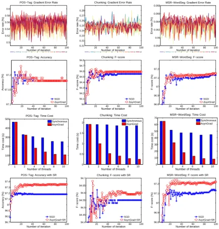
Figure 2: Experimental results on dense-CRF. For the 1st row, 1 to 10 denote the 10 threads ofAsynGrad. For the 2nd row,AsynGraddenotesAsynGradwith 10 threads.
traditional implementation of CRF, usually the edges features contain only tag transitions with the form
(yi−1, yi). In dense-CRF, we incorporate local tokens ofxxx into the edge features, which is called rich
edge features (Sun et al., 2012; Sun et al., 2014). For example, a rich edge feature can be(xi, yi−1, yi)
or even(xi−1, xi, yi−1, yi). A simple way to automatically create massive rich edge features is to extend
each node feature (x, yi) to the rich edge feature (x, yi−1, yi), where x means the tokens of a local
window. Usually a naive way to do this will cause feature explosion. However, it is easy to solve this problem — only extend high frequency node features (e.g., frequency larger than 10) to rich edge features. In many real-world tasks we find this type of dense-CRF works much better than traditional CRF, and without feature explosion problem even for tasks with many tags (e.g., the POS tagging task). The standard SGD learning method (Bertsekas, 1999; Bottou and Bousquet, 2008; Shalev-Shwartz and Srebro, 2008) is chosen as the baseline. Based on tuning, the initial learning rate of SGD is set as 0.02, 0.05, 0.1 for the POS-Tag, Chunking, and MSR-WordSeg tasks, respectively. To control overfitting, we use theL2regularizer, i.e., a Gaussian prior. TheL2regularization strength (i.e., the termλ) is set as
1, 0.5, 1 for the three tasks, respectively.
5 10 15 20 90 92 94 96 98 100
Number of iteration
Error Rate (%)
POS−Tag: Gradient Error Rate
1 2 3 4 5 6 7 8 9 10
5 10 15 20
90 92 94 96 98 100
Number of iteration
Error Rate (%)
Chunking: Gradient Error Rate
1 2 3 4 5 6 7 8 9 10
5 10 15
90 92 94 96 98 100
Number of iteration
Error Rate (%)
Weibo−WordSeg: Gradient Error Rate
1 2 3 4 5 6 7 8 9 10
10 20 30 40 50
94 94.5 95 95.5 96 96.5 97 97.5
Number of iteration
Accuracy (%)
POS−Tag: Accuracy
Adam AsynGrad
0 10 20 30 40 50
94 94.5 95 95.5
Number of iteration
F−score (%)
Chunking: F−score
Adam AsynGrad
0 10 20 30 40 50
89 89.5 90 90.5 91 91.5 92 92.5 93
Number of iteration
F−score (%)
Weibo−WordSeg: F−score
Adam AsynGrad
1 2 4 6 8 10
0 500 1000 1500 2000 2500 3000
Number of threads
Time cost (s)
POS−Tag: Time Cost
Synchronous AsynGrad
1 2 4 6 8 10
0 500 1000 1500 2000
Number of threads
Time cost (s)
Chunking: Time Cost
Synchronous AsynGrad
1 2 4 6 8 10
0 500 1000 1500 2000
Number of threads
Time cost (s)
Weibo−WordSeg: Time Cost
[image:7.595.85.516.63.401.2]Synchronous AsynGrad
Figure 3: Experimental results on LSTM. For the 1st row, 1 to 10 denote the 10 threads ofAsynGrad. For the 2nd row,AsynGraddenotesAsynGradwith 10 threads.
Table 2: Some major experimental results on LSTM. Time means time cost per iteration. Method Acc (%) Time (s) F-score (%) Time (s) F-score (%) Time (s)POS-Tag Chunking Weibo-WordSeg
Adam 96.40 2972.13 95.40 1750.68 91.79 2198.45
AsynGrad(10-thread) 96.77 793.40 95.45 465.95 91.93 607.22
among total gradients. For example, if a thread used 100 gradients and 5 gradients are with errors in this iteration, its gradient error rate is 5%. As we can see, the gradient errors are not rare in asynchronous parallel learning.
The 2nd row shows the accuracy/F-score curves. As we can see, when facing the gradient errors, the proposed asynchronous parallel learning methodAsynGrad has no loss at all on the accuracy/F-score, compared with traditional SGD (single thread).
The 3rd row shows the speed acceleration ofAsynGrad, compared with synchronous parallel learning method (Langford et al., 2009). As we can see, when adding more threads for parallel learning,AsynGrad achieves substantially better acceleration on the training speed than the synchronous parallel learning method.
The 4th row shows the accuracy/F-score curves by combiningAsynGradwith structure regularization (SR) (Sun, 2014). SR is a simple method to prevent overfitting by splitting samples into mini-samples, thus it reduces the complexity and sparsity of structures (Sun, 2014). As we can see, AsynGrad can easily combine with SR to improve the accuracy/F-score on those tasks.
[image:7.595.80.517.467.530.2]3.2 Experiments on LSTM (Completely Dense Case)
Recently, long short term memory networks (LSTM) has widely applied to many tasks (Chen et al., 2015; Hammerton, 2003; Cho et al., 2014). In this work, we use the bi-directional long short term memory network (Bi-LSTM) as the implementation of LSTM, which has better accuracy than single-directional LSTM in many practical tasks. The LSTM recurrent cell is controlled by three “gates”, namely input gate, forget gate and output gate.
Adaptive learning versions of SGD are popular to train large neural networks, including the Adam learning method (Kingma and Ba, 2014), the RMSProp learning method (Tieleman and Hinton, 2012), and so on. The experiments on LSTM are based on the Adam learning method, with the hyper parameters as follows: β1 = β2 = 0.95, ϵ = 1×10⁻⁴ (Kingma and Ba, 2014). The input/hidden dimension is
170, 280, and 220 for the POS-Tag, Chunking, and Weibo-WordSeg tasks, respectively. For the tasks with LSTM, we find there is almost no difference on the results by adding L2 regularization or not.
Hence, we do not addL2regularization for LSTM. All weight matrices, except for bias vectors and word
embeddings, are diagonal matrices and randomly initialized by normal distribution.
The experimental results are shown in Figure 3. The 1st row shows the percentage of gradient errors among total gradients. As we can see, for neural networks like LSTM, the gradient errors are very common (the rate is over 90%) in asynchronous parallel learning. The gradient error rate is much higher than the CRF case, this is because the LSTM is a much more dense model compared with dense-CRF. In fact, LSTM can be seen as a completely dense model because there is totally no sparse feature existing.
The 2nd row shows the accuracy/F-score curves. As we can see, when facing the intensive gradient errors which are over 90% on very dense models like LSTM,AsynGradhas no loss at all on accuracy/F-score.
The 3rd row shows the speed acceleration ofAsynGrad, compared with synchronous parallel learning method (Langford et al., 2009). As we can see, when adding more threads for parallel learning,AsynGrad achieves substantially better acceleration on the training speed than the synchronous version.
The experiments shows thatAsynGradcan substantially accelerate the training speed of LSTM, and without any loss on accuracy. Some major experimental results are summarized in Table 2.
4 Proof
Here we give the proof of Theorem 1. First, the recursion formula is derived. Then, the bounds are derived.
4.1 Recursion Formula
By subtractingwww∗from both sides and taking norms for (1), we have
||wwwt+1−www∗||2=||wwwt−γssszzzt(wwwt)−www∗||2
=||wwwt−www∗||2−2γ(wwwt−www∗)Tssszzzt(wwwt) +γ2||ssszzzt(wwwt)||2
(12)
Taking expectations and letat=E||wwwt−www∗||2, we have
at+1=at−2γE[(wwwt−www∗)Tssszzzt(wwwt)] +γ2E[||ssszzzt(wwwt)||2]
(based on (6) )
≤at−2γE[(wwwt−www∗)Tssszzzt(wwwt)] +γ2κ2
(since the random draw ofzzztis independent ofwwwt)
=at−2γE[(wwwt−www∗)TEzzzt(ssszzzt(wwwt))] +γ2κ2
=at−2γE[(wwwt−www∗)Tsss(wwwt)] +γ2κ2
(13)
We define
and insert it into (4), it goes to
f(www′)≥f(www) + (www′−www)T[sss(www) +δ(www)] + c
2||www′−www||2
=f(www) + (www′−www)Tsss(www) +c2||www′−www||2+ (www′−www)Tδ(www) (15)
By settingwww′ =www∗, we further have
(www−www∗)Tsss(www)≥f(www)−f(www∗) +c2||www−www∗||2−(www−www∗)Tδ(www)
≥ 2c||www−www∗||2−(www−www∗)Tδ(www) (16)
Combining (13) and (16), we have
at+1 ≤at−2γE
[c
2||wwwt−www∗||2−(wwwt−www∗)Tδ(wwwt)
]
+γ2κ2
= (1−cγ)at+ 2γE[(wwwt−www∗)Tδ(wwwt)] +γ2κ2
(17)
Considering (8) and (14), it goes to
at+1≤(1−cγ)at+ 2γτ+γ2κ2 (18)
We can find a steady statea∞by the formulaa∞= (1−cγ)a∞+ 2γτ+γ2κ2, which gives
a∞= 2τ+γκ
2
c (19)
Defining the functionA(x) = (1−cγ)x+ 2γτ+γ2κ2, based on (18) we have
at+1≤A(at)
(Taylor expansion ofA(·)based ona∞, with∇2A(·)being 0)
=A(a∞) +∇A(a∞)(at−a∞)
=A(a∞) + (1−cγ)(at−a∞)
=a∞+ (1−cγ)(at−a∞)
(20)
Thus, we haveat+1−a∞≤(1−cγ)(at−a∞), and unwrapping it goes to
at≤(1−cγ)t(a0−a∞) +a∞ (21)
4.2 Bounds
Since∇f(www)is Lipschitz according to (5), we have
f(www)≤f(www′) +∇f(www′)T(www−www′) + q2||www−www′||2
Settingwww′=www∗, it goes tof(www)−f(www∗)≤ q
2||www−www∗||2, such that
E[f(wwwt)−f(www∗)]≤ 2qE||wwwt−www∗||2 = q2at
In order to haveE[f(wwwt)−f(www∗)]≤ϵ, it is required thatq2at≤ϵ, that is
at≤ 2qϵ (22)
Combining (21) and (22), it is required that
To meet this requirement, it is sufficient to set the learning rateγsuch that both terms on the left side are less than ϵ
q. For the requirement of the second terma∞≤ qϵ, recalling (19), it goes toγ ≤ cϵ−qκ22τq. Thus,
introducing a real valueβ≥1, we can setγ as
γ = cϵ−2τq
βqκ2 (24)
Note that, to make this formula meaningful, it is required thatcϵ−2τq≥0. Thus, it is required that
τ ≤ cϵ
2q
which is solved by the condition of (11).
On the other hand, we analyze the requirement of the first term that(1−cγ)t(a0−a∞) ≤ ϵ q. Since a0−a∞≤a0, it holds by requiring(1−cγ)ta0 ≤ ϵq, which goes to
t≥ log
ϵ qa0
log (1−cγ) (25)
Sincelog (1−cγ)≤ −cγgiven (7), and thatlog ϵ
qa0 is a negative term, we have
log ϵ qa0
log (1−cγ) ≤ log ϵ
qa0
−cγ
Thus, (25) holds by requiring
t≥ logqaϵ0
−cγ =
log (qa0/ϵ)
cγ (26)
Combining (24) and (26), the problem can be addressed as far as
t≥ βqκc(2cϵlog (−2qaτq0)/ϵ)
Thus, settingt .= βqκ2log (qa0/ϵ)
c(cϵ−2τq) can solve the problem. This completes the proof. ⊓⊔
5 Conclusions
In this paper we show that gradient errors are very common and inevitable in dense feature models. Nevertheless, we show that the learning process with the gradient error problem can still approach the optimum in many practical applications. We propose a simple method AsynGrad for asynchronous stochastic parallel learning with gradient error. We show thatAsynGrad works well for dense feature models like neural networks and dense-CRF, in spite of gradient errors. Base on various NLP tasks, our experiments show thatAsynGrad can substantially accelerate the training speed of LSTM and dense-CRF, and without any loss on accuracy.
Acknowledgements
References
D.P. Bertsekas. 1999. Nonlinear Programming. Athena Scientific.
L´eon Bottou and Olivier Bousquet. 2008. The tradeoffs of large scale learning. InNIPS’08, volume 20, pages 161–168.
Xinchi Chen, Xipeng Qiu, Chenxi Zhu, Pengfei Liu, and Xuanjing Huang. 2015. Long short-term memory neural networks for chinese word segmentation. In Llu ´ıs M `arquez, Chris Callison-Burch, Jian Su, Daniele Pighin, and Yuval Marton, editors,EMNLP, pages 1197–1206. The Association for Computational Linguistics. KyungHyun Cho, Bart van Merrienboer, Dzmitry Bahdanau, and Yoshua Bengio. 2014. On the properties of
neural machine translation: Encoder-decoder approaches. CoRR, abs/1409.1259.
Michael Collins. 2002. Discriminative training methods for hidden markov models: Theory and experiments with perceptron algorithms. InProceedings of EMNLP’02, pages 1–8.
Jeffrey Dean, Greg Corrado, Rajat Monga, Kai Chen, Matthieu Devin, Quoc V. Le, Mark Z. Mao, Marc’Aurelio Ranzato, Andrew W. Senior, Paul A. Tucker, Ke Yang, and Andrew Y. Ng. 2012. Large scale distributed deep networks. InProceedings of NIPS, pages 1232–1240.
Ofer Dekel, Ran Gilad-Bachrach, Ohad Shamir, and Lin Xiao. 2012. Optimal distributed online prediction using mini-batches. Journal of Machine Learning Research, 13:165–202.
Jianfeng Gao, Galen Andrew, Mark Johnson, and Kristina Toutanova. 2007. A comparative study of parameter estimation methods for statistical natural language processing. InProceedings of ACL’07, pages 824–831. Kevin Gimpel, Dipanjan Das, and Noah A. Smith. 2010. Distributed asynchronous online learning for natural
language processing. In Mirella Lapata and Anoop Sarkar, editors,Proceedings of CoNLL, pages 213–222. James Hammerton. 2003. Named entity recognition with long short-term memory. In Walter Daelemans and
Miles Osborne, editors,CoNLL, pages 172–175. ACL.
Diederik Kingma and Jimmy Ba. 2014. Adam: A method for stochastic optimization. arXiv preprint arX-iv:1412.6980.
John Langford, Alex J. Smola, and Martin Zinkevich. 2009. Slow learners are fast. InNIPS’09, pages 2331–2339. Brendan Mcmahan and Matthew Streeter. 2014. Delay-tolerant algorithms for asynchronous distributed online
learning. InAdvances in Neural Information Processing Systems 27, pages 2915–2923.
Feng Niu, Benjamin Recht, Christopher Re, and Stephen J. Wright. 2011. Hogwild: A lock-free approach to parallelizing stochastic gradient descent. InNIPS’11, pages 693–701.
Benjamin Recht and Christopher Re. 2013. Parallel stochastic gradient algorithms for large-scale matrix comple-tion. Math. Program. Comput., 5(2):201–226.
Erik Tjong Kim Sang and Sabine Buchholz. 2000. Introduction to the CoNLL-2000 shared task: Chunking. In Proceedings of CoNLL’00, pages 127–132.
Shai Shalev-Shwartz and Nathan Srebro. 2008. Svm optimization: inverse dependence on training set size. In ICML’08, pages 928–935. ACM.
Xu Sun, Louis-Philippe Morency, Daisuke Okanohara, and Jun’ichi Tsujii. 2008. Modeling latent-dynamic in shallow parsing: A latent conditional model with improved inference. InProceedings of COLING’08, pages 841–848, Manchester, UK.
Xu Sun, Houfeng Wang, and Wenjie Li. 2012. Fast online training with frequency-adaptive learning rates for chinese word segmentation and new word detection. InProceedings of ACL’12, pages 253–262.
Xu Sun, Wenjie Li, Houfeng Wang, and Qin Lu. 2014. Feature-frequency-adaptive on-line training for fast and accurate natural language processing. Computational Linguistics, 40(3):563–586.
Xu Sun. 2014. Structure regularization for structured prediction. InAdvances in Neural Information Processing Systems (NIPS), pages 2402–2410.
Tijmen Tieleman and Geoffrey Hinton. 2012. Lecture 6.5: rmsprop: divide the gradient by a running average of its recent magnitude. InCOURSERA: Neural Networks for Machine Learning.