Division V
CONSTANT-DUCTILITY FLOOR RESPONSE SPECTRUM AND
APPLICATION FOR DYNAMIC ANALYSIS OF
INELASTIC MULTI-DEGREE-OF-FREEDOM SYSTEMS
Ichiro Tamura1 and Shinichi Matsuura2
1
Manager, The Chugoku EPCO, Hiroshima, Japan ([email protected]) 2
Senior Research Engineer, Central Research Institute of Electric Power Industry, Chiba, Japan
ABSTRACT
A constant-ductility response spectrum (CDRS) readily provides the yield strength (or yield deformation) necessary to limit the ductility imposed by a ground motion to a specified value in a single-degree-of-freedom (SDF) system. This spectrum is central to understanding the earthquake response and design of yielding structures and components. The allowance of inelastic deformation of the SDF system leads to reduction of the required yield strength. In this study, we discussed inelastic behavior of SDF systems located on floors by investigating CDRS for floor motions amplified by the structures, and indicated that the yield strength required of the system would be simply obtained with increasing values of ductility factor. We also discussed a dynamic analysis method of inelastic multi-degree-of-freedom (MDF) systems based on a spectrum modal analysis by using the CDRS.
CONSTANT-DUCTILITY RESPONSE SPECTRUM
Equation of Motion for Inelastic SDF Systems
We considered an inelastic single-degree-of-freedom (SDF) system that has a restoring force of a bilinear skeleton curve, as shown in fig. 1, with kinematic hardening type. The equation of motion for elastic region of the system is
) ( )
(t x xy
F kx x c x
m (1)
where x is the deformation, m is the mass, c is the damping coefficient, k is the elastic stiffness, t is time, F(t) is the external force and xy is the yield deformation. Yielding begins at the deformationxy, and the system becomes plastic with the second stiffnessk'. The equation of motion for plastic region of the system is
) ( ) ( ) ' (
'x k k xy F t x xy k
x c x
m (2)
Dividing Equations 1 and 2 by m gives
) ( 2h x 2x xE x xy
x
(3)
) ( )
' ( '
2h x 2x 2 2 xy xE x xy
x
(4)
where k m is the elastic natural frequency, ' k' m is the natural frequency corresponding to second stiffness, hc 2 mkis the damping ratio and xE F(t) m is the acceleration of the external force. To obtain the equations of motion for the system expressed in term of the ductility factor, dividing Equations 3 and 4 by xy give
) ( 2h 2 2xE ay xxy
(5)
) ( )
' ( '
2h 2 2 2 2xE ay xxy
where x xyis the time-dependent ductility factor and ay 2xy is the yield acceleration of the system. Equations 5 and 6 demonstrate that the ductility factor max
(t)
depends on four system parameters: ay,Tn,,h for a given xE, where Tn 1
is the natural period, k' k is the stiffness ratio. Herein ay can be replaced with f y or xy, where f ymay is the yield strength of the system.Figure 1. Load-deformation diagram of inelastic SDF system
Constant-Ductility Response Spectrum
For a given external forceF(t), the constant-ductility response spectrum (CDRS) is a plot showing yield strength fy of SDF systems as a function of natural periodTn for a fixed ductility factor, stiffness ratio and damping ratioh. Herein we defined the normalized yield strength as the yield strength fy divided by the maximum external forceF0, that is the maximum value of F(t):
0 0
0 x
x A a F
fy y y
(7)
where A0F0 m is the zero period acceleration (ZPA), x0 F0 k is the deformation, respectively, in the corresponding elastic system by the maximum external forceF0. The CDRS is also expressed in terms of the normalized yield strength instead of the yield strengthf y. The normalized yield strength can be written in terms of the corresponding normalized yield strength0 of the rigid system as follows:
) 1 ( 1
) , , , ( ) , ( ) , , , ( ) , , ,
( 0
R T h R T h
h
T n
n
n (8)
where we defined the response factorR 0.
Veletsos and Newmark (1960), Veletsos et al. (1965) and Veletsos (1969) indicated below results by calculating CDRS of elastic-perfectly-plastic systems, which were well summarized in Chopra (2011). The yield strength f y required of an SDF system permitted to undergo inelastic deformation is less than minimum strength necessary for the structure to remain elastic. The required yield strength f y is reduced with increasing values of the ductility factor. Even small amounts of inelastic deformation, corresponding to1.5, produce a significant reduction in the required yield strengthf y. Additional reductions are achieved with increasing values of the ductility factor but at a slower rate. And the required yield strength f y for a specified ductility factor also depends on the damping ratioh, but this dependence is not strong.
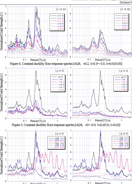
We referred to a CDRS for a floor motion as a constant-ductility floor response spectrum (CDFRS). Figures 4 and 5 show the CDFRS calculated by the Western-Tottori Earthquake (2000.10.06) floor-acceleration record, as shown in Fig. 2, observed at Shimane NPPs Unit2(NS-2) reactor-building(R/B) (first natural periodTB :0.22s) which was amplified by the structure. From these figures,
y
f
Q
x
y
x
k
'
k Plastic region
Elastic region Corresponding
we verified that the same indicated by Veletsos and Newmark was equally true of fy--h relations excluding about equal to unity for elasto-plastic SDF systems located on the floors. Increasing values of ductility factor connect to increasing three system/response parameters: (1) hysteresis damping of the response, (2) strength(1( 1))fy and (3) deformationxy of an inelastic system. Increasing of these parameters reduces the required yield strengthf y, and the reduction effect of each parameter depends on the natural periodTn and the stiffness ratio for a specified ductility factor. We summarized behavior of inelastic SDF systems to Table 1 by investigating the CDFRS of Fig. 4, 5 and others. Figure 3 is the schematic diagram of CDFRS for a characteristic floor motion.
Hereafter we discussed behavior of the systems with 0Tn 2TB in the amplification significant region of corresponding elastic systems, where is the main periodic band of NPPs components. The yield strengths fy required of these systems are reduced with increasing values of (1) hysteresis damping and (2) strength in the three system/response parameters. In the limit as tends to zero, (1) hysteresis damping effect will be maximum and (2) strength effect will be minimum (disappeared). On the other hand, in the limit as tends to unity, the former one will be minimum (disappeared) and the latter one will be maximum. Thus, in the intermediate range of , the reduction of the yield strengths f y of these systems is due to both effects for a specified ductility factor .
We verified that (1) hysteresis damping reduced the response factorR to near by unity with increasing values of the ductility factor, excluding about equal to unity. Even small amounts of inelastic deformation produced a significant reduction in the response factorR. Additional reductions of the response factorR were achieved with increasing values of the ductility factor but at a slower rate. Thus, the natural periodTn and the damping ratioh dependence for the response factorR would be loosed by increasing values of the ductility factor for a specified stiffness ratio. As a result, the normalized yield strength could be conservatively and reasonably approximated as shown in Equations 9 and 10.
) , ( ) , ( ' ) , ( ' ) , , ,
( 0
Tn h R (9)
R Tn h Tn TB
R'(,)max (, ,, 0.01); 0 2 (10)
where the damping ratioh=0.01 is the conservative one of components. For example, from Figure 4, the required normalized yield strength can be approximated by unity regardless of the natural periodTn if ductility factor of three is allowed at an inelastic system with stiffness ratio of 0.2. Figure 6 shows the CDFRS calculated by the records mentioned before and the Niigata-Chuetsu-Oki Earthquake (2007.7.16) floor-acceleration record observed at Kashiwazaki-Kariwa NPPs Unit7(KK-7) R/B(first natural period
B
T :0.42-0.43s) provided by TEPCO, as shown in Fig. 2. We verified that loss of the natural period dependence meant loss of the external forceF(t) dependence for the normalized yield strength from Fig. 6. Under this condition, the required yield strength f y depends on just the maximum external forceF0in the time history of external forceF(t).
Excluding the stiffness ratio about equal to unity, the stiffness ratio dependence for the normalized yield strength is not so strong. In many case, it is difficult to know the stiffness ratioexactly. But if the minimum and maximum stiffness ratiomin,max can be roughly estimated, the normalized yield strength could be conservatively approximated for a specified ductility factor as shown in Equation 11.
'( , ); min max
max ) ( ' ' ) , , ,
(
Table 1: Behavior of inelasticSDF systems for a specified ductility factor
Normalized yield strength
) , , , ( Tn h
Reduction effect (ratio) from elastic normalized yield strengthE(Tn,h)*1 Natural
Period
n
T 0 :0 1
1 Hysteresis Damping Strength0 1 1 ( 1)
1
1
Non
B T
2 0
, ,
( T
R
) , 0 h
1( 1) ) , , , (
h T
R n Ris quickly reduced until 1, after that,
R is slowly reduced with increasing values of for a specified(1).
1) ( 11
B T
2 App. EBASE(Tn,h)
E(Tn,h)
E
is quickly reduced untilEBASE*2. 1
*4*1 E(T,h)(1,Tn,h) *2 EBASE(Tn,h) is the base line of E(Tn,h) as shown in Figure 3. *3 (,Tn,,h) : For a specified , is reduced with increasing value of from zero to because
of the strength increasing. After that, is increased with increasing value of from to unity because of decrease of hysteresis damping. (0 1) gives the local minimal value of .
*4 The reduction cause is deformation increasing, not strength increasing. T ime(s)
T ime(s)
Figure 2. History waveforms of floor response The Niigata-Chuetsu-Oki Earthquake at KK-7 R/B ch7R-1
*3
MAX=435cm/s2 MAX=-48.0m/s2 The Western-Tottori Earthquake at NS-2 R/B ch24
A
cc
el
er
at
io
n
(
c
m
/s
2)
A
c
cel
er
at
io
n
(
cm
/s
2)
T ime(s)
The Western-Tottori Earthquake at NS-2 R/B ch26
A
cce
le
rat
io
n
(
cm
/s
2) MAX=-48.7m/s
2
Figure 4. Constant ductility floor response spectra [ch24, γ=0.2, μ=1.0 5.0, h=0.01/0.05]
N
o
rm
al
ized
Y
ie
ld
S
tr
en
g
th
[
χ
]
Period [T] (s)
Figure 5. Constant ductility floor response spectra [ch24, γ=0 0.9, μ=2.0/5.0, h=0.02]
Figure 6. Constant ductility floor response spectra [NS-2ch24/26/KK-7ch7R-1, γ=0.2, μ=2.0/5.0, h=0.02] Period [T] (s)
N
o
rm
al
ized
Y
ie
ld
S
tr
en
g
th
[
χ
]
N
o
rm
al
ized
Y
ie
ld
S
tr
en
g
th
[
χ
]
Period [T] (s) Period [T] (s)
APPLICATION FOR DYNAMIC ANALYSIS OF INELASTIC MDF SYSTEMS
Modal Expansion of Elastic MDF Systems
We considered an elastic N-degree of freedom (DOF) system. The equations of motion are
M
X
C
X
K
X
M
XE (12)where
TE E
E E T
N X x x x
x x
x
X 1 2 , (13)
ji ij ij
ij N
j ij
ii k i N K k i j i N j N k k
K
), 1 , 1 , ( ),
1 ( 1
(14)
X is the deformation vector,
M is the mass matrix of mass 1~N(m1~mN),
C is the classical damping matrix,
K is the stiffness matrix of the system, kij is the stiffness of mass i - j interaction(i,j1~N) and
XE is the acceleration vector of the external forceF(t). We defined the modal matrix
, each column of which is the natural mode
i
i , corresponding to the natural frequencyi of the system. The deformation vector
X of the N-DOF system can be expressed, as shown in Equation 15, as the superposition of the modal contributions:
TN N
N q q q q q
q q
q
X 11 22 , ( 1 2 ) (15)
Equations 12 and 15 give the equation of motion in modal coordinateqr, as shown in Equation 16.
E r r r r r r
r h q q x
q
2
2 (16)
where hr is the damping ratio and r is the modal participation factor for rth mode. Dividing Eq-uation 16 by r gives the equation of motion in modal coordinater qr/r, as shown in Equation 17.
E r r r r r
r h x
2
2 (17)
Developed Method of Simplified Dynamic Analysis of Inelastic MDF Systems by Using CDRS
We considered an inelastic N-DOF system (e.g., Fig. 9), each interaction of massi- j has a restoring force of a bilinear skeleton curve, as shown in Figure 1, with kinematic hardening type. The equations of motion for elastic region( xixj xijy) of the system are equal to Equations 12, 16 and 17, where xijy is the yield deformation of massi- j interaction(i,j1 N).
We assumed first yielding of the system begins at mass1-1interaction when the deformation reaches xy11, second yielding of the system begins at mass2-2 interaction when the deformation reaches xy22,…and final yielding of the system begins at massn-n interaction when the deformation reaches xynn in a cycle of motion. Then the yielding interaction of massi- j becomes plastic with stiffnessk' . The equations of motion for partially plastic region of the system are ij
Ey n
n y n n n
n X K K X K K X M X
K X C X
M ( 1 1)( ) ( ) ( ) ( 1 1) ( 1 1)
) ' (
) ' (
'
))) ( , ), (( ) , ( )),
( , ), (( ) , (
( xixj xijy i j 11 nn xixj xijy i j 11 nn (18) where
yij j i T j
i ij
y x x x x x
)) ( , ), ( ) , (( ' , ' ' ), ( ' ' , '
' 1 1
1 n n ij ij ji ij ij ij N j ij
ii k K k i j k k k k i j
K
(20)
We introduced the yield deformation of massi- j interaction in modal coordinates qry(ij) as follows:
rj ri y ij ij y r x q ) ( (21)
Premultiplying each term in Equation 18by
T, substituting Equation 15 in Equation 18 and using Equation 21 give equation of motion in modal coordinatesqr, as shown in Equation 22.E r y r r rr r n n y r r n n rr r N s s r n n rs r r r
r q x
M K K q M K K q M K q h
q
) 1 1 ( ) 1 1 ( ) ( ) ( 1 ) ( ) 1 1 ( ' ' '2 (22)
where
r T
r r
r T
r rs n n
r T
n n
sr M K K K K
M , , '(11)( ) '(11)( ) (23) To simplify Equation 22, we assumed
) ( 0 '( 1 1) ( ) r s
Krs nn
(24)
This assumption gives
E r y r rr r n n y r n n rr r r n n rr r r r
r h q q q q x
q (11)( )2 2( )2 ( ) 2(11)2 (11)
) ' ( ) ' ( '
2 (25)
where r2Kr/Mr, 'rr nn K'(rr11) (nn)/Mr 2 ) ( ) 1 1 (
. Dividing Equation 25 by r givesequation of motion in modal coordinatesr, as shown in Equation 26.
E y r rr r n n y r n n rr r r n n rr r r r
r h x
( 1 1)( )2 2 ( )2 ( ) 2 ( 1 1)2 ( 1 1) ) ' ( ) ' ( '
2
(26)
where r
ij y r ij y
r q
( ) ( )
. Equation 26 indicates that the subsystem of modal coordinatesr has the restoring force of the multi-linear skeleton curve with kinematic hardening type. To simplify the restoring force, we approximated the multi-linear skeleton curve to the bilinear skeleton curve of which the elastic stiffness is Kr and the second stiffness is K''r with kinematic hardening type as shown in Fig. 7.
Figure 7. Load-deformation diagram of original and approximated r-subsystem ) ( ) 1 1 (
' rr i i
K
r K ) 1 1 ( 'rr
K ) ( ) 1 1 (
' rr n n
K
) ( i i
y r
y( n n)r
max r r
rK ''
This approximation gives E y r r r r r r r r
r h x
2 2 2 ( 1 1)
) ' ' ( ' '
2
(27) where r r r r M K '' '' ( ) max 2 (28) max r
is the maximum deformation of r, K''r is the function of rmax, and Equations 17 and 27 give max
r
. Thus, rmax is obtained by convergence calculation. To obtain the equation of motion expressed in term of the ductility factor in modal coordinater, dividing Equations 17 and 27 by
ry(11) give) 1 1 ( 2 ) 1 1 ( 2 ) 1 1 ( ) 1 1 (
2
y r E r r r r r r
r h x a
(29) ) 1 1 ( 2 2 2 ) 1 1 ( 2 ) 1 1 ( ) 1 1
( 2 '' ( '' )
y r E r r r r r r r r
r h x a
(30)
where r(11)(t)r(t) ry(11) and ay(r11)r2ry(11). The ductility factor of the rth mode for mass1-1 interaction, r(11) max
r(11)(t)
is expressed as) , , , ( ( 1 1) ) 1 1 ( r r r y r
r a T h
(31) where ) ( 1 1
1 1 2 ) 1 1 ( 2 ) 1 1 ( 2 ) 1 1 ( r r r y r r y r r y r r y r x q a , r r T 1 , r r r r K K
'' ( max) (32)
Equations 29 and 30 are the same as Equations 5 and 6. Therefore, the ductility factor r(11) is obtained
from the yield acceleration ay(r11) and the natural period Tr by using the CDRS of which the stiffness
ratio is rand the elastic damping is hr. The ductility factorr(ij) of the rth mode for massi- j interaction is expressed as follows:
( ) ) 1 1 ( ) 1 1 ( ) ( ) 1 1 ( ) 1 1 ( ) ( )( max () max ()
ij y r y r r ij y r y r r ij r ij
r t t
(33)
The time-dependent ductility factorx(ij) of massi - j interaction is expressed by q(ij) r
or r(ij)as follows: ) ( ) ( ) ( ( ) ( ) )
( t t t
r ij r r ij q r ij
x
(34)
The ductility factorx(ij)of massi- j interaction is approximately obtained by modal combination rules as shown in Equation 35.
ABSSUM
r ij r ij
x( ) ( )
, SRSS
r ij r ij
x( ) ( ) 2 ) (
(35)
Dynamic Analysis of Inelastic 2-DOF Systems by the Developed Method
We calculated the ductility factor of the 2-DOF systems by the developed method (DM). Figures 9 and 10 show the calculated models and the vibration modes of the 2-DOF systems (m1m2 1kg,
k k
k11 12 , k22 2k, f11y f12y f22y 2N, 0.2, h0.02). We calculated for five cases of external forces with the acceleration record (NS-2 R/B ch24) multiplied by factors. The First level is the elastic limit of the system, and the others are the levels of external forces multiplied the elastic limit by 1.5, 2, 3, 6. The first yielding and maximum deforming interaction was m2-floor interaction.
Figure 8. Comparison of calculated ductility factors
M odel B:m2-Floor Interaction
M odel B:m1-m2 Interaction
M odel B: m1-Floor Interaction
M odel C:m2-Floor Interaction
M odel C:m1-m2 Interaction
M odel C:m1-Floor Interaction
M odel A:m2-Floor Interaction
M odel A:m1-m2 Interaction
Figure 8 shows the calculated ductility factors of the systems by the DM using CDFRS (e.g., Fig.5), one of those by the response history analysis (RHA) and one of the corresponding elastic systems by the spectrum modal analysis (SMA). The ratios of the ductility factor of each interaction by the DM with ABSSUM to one by the RHA is over 0.95 at Model A, 0.8 at Model B and 0.7 at Model C in these calculated results, that involve not only one interaction yielding but also two or three interaction yielding of each model. These results indicate that the vibration modes of elastic regions hold good for the above calculated inelastic conditions. The developed method is effective as a dynamic analysis method of inelastic MDF systems in these conditions, and is also considered of value for understanding earthquake responses of inelastic MDF systems by spectrum modal approaches.
Model Model A Model B Model C
k 230 N/m 600 N/m 1000N/m
1st Tn 0.35s Not Peak
0.22s 1st Peak
0.17s Not Peak 2ndTn 0.22s
1st Peak
0.13s 2nd Peak
0.10s Not Peak
CONCLUSION
By investigating CDRS for floor motions, we verified that the yield strength required of an SDF system located on a floor was reduced with increasing values of the allowance of inelastic deformation. The reduction is significant in the natural period band where the floor response is widely amplified by the structure. In consequence, increasing values of the ductility factor lead the required yield strength less sensitive to the natural period of the SDF system and that is represented by a value of the ZPA multiplied by the mass, regardless of time history of the external force. Moreover, we developed a simplified method based on a spectrum modal analysis using CDRS as a dynamic analysis method of inelastic MDF systems, and we verified that was effective in the calculated 2-DOF systems. This method is considered of value for understanding earthquake responses of inelastic MDF systems by spectrum modal approaches.
REFERENCES
Chopra, A. K. (2011). Dynamics of Structures, 4th ed., Prentice Hall, New Jersey, USA, pp.257-305. Tamura, I. and Matsuura, S. (2011). Consideration of Elasto-Plastic Behavior of Components Based on
Elasto-Plastic Response Spectrum, Proceedings of the JSME Dynamics and Design Conference, Kochi, Japan, No.512.
Veletsos, A. S. and Newmark, N. M. (1960). Effect of Inelastic Behavior on the Response of Simple Systems to Earthquake Motions, Proceedings of the 2nd World Conference on Earthquake Engineering, Japan, Vol.2, pp.895-912.
Veletsos, A. S., Newmark, N. M. and Chelapati, C.V. (1965). Deformation Spectra for Elastic and Elastoplastic Systems Subjected Ground Shock and Earthquake Motion,” Proceedings of the 3rd World Conference on Earthquake Engineering, New Zealand, Vol.II, pp.663-682.
Veletsos, A. S. (1969). Maximum Deformation of Certain Nonlinear Systems,” Proceedings of the 4th World Conference on Earthquake Engineering, Santiago, Chile, Vol. 1, pp.155-170.
Elastic
k
11k
12k
221
m
m
2Plastic
k
'
11k
'
12k
'
22Figure 10. Vibration modes of the 2-DOF system Figure 9. Inelastic 2-DOF system
1
0.618 1