A new model for the estimation of cell proliferation dynamics using CFSE data

(1)

A New Model for the Estimation of Cell Proliferation Dynamics Using

CFSE Data

H.T. Banks, Karyn L. Sutton and W. Clayton Thompson

Center for Research in Scientific Computation and Center for Quantitative Sciences in Biomedicine

North Carolina State University, Raleigh, NC 27695-8212

Gennady Bocharov

Institute of Numerical Mathematics, RAS, Moscow, Russia

Marie Doumic

INRIA Rocquencourt, Projet BANG, Domaine de Voluceau, 78153 Rocquencourt, France

Tim Schenkel

1

, Jordi Argilaguet

2

, Sandra Giest

2

, Cristina Peligero

2

and Andreas Meyerhans

1,2

1_{Department of Virology, Saarland University, D-66421 Homburg, Germany}

and

2_{ICREA Infection Biology Lab, Dept of Experimental and Health Sciences, Univ. Pompeu Fabra, 08003 Barcelona, Spain}

August 20, 2011

Abstract

CFSE analysis of a proliferating cell population is a popular tool for the study of cell division and division-linked changes in cell behavior. Recently [13, 45, 47], a partial differential equation (PDE) model to describe lymphocyte dynamics in a CFSE proliferation assay was proposed. We present a significant revision of this model which improves the physiological understanding of several parameters. Namely, the parameterγ used previously as a heuristic explanation for the dilution of CFSE dye by cell division is replaced with a more physical component, cellular autofluorescence. The rate at which label decays is also quantified using a Gompertz decay process. We then demonstrate a revised method of fitting the model to the commonly used histogram representation of the data. It is shown that these improvements result in a model with a strong physiological basis which is fully capable of replicating the behavior observed in the data.

Key words: Cell proliferation, cell division number, CFSE, label structured population dynamics, partial

(2)

1 Introduction

The quantitative analysis of cell division is an important problem at the intersection of biology and mathemat-ics. Of the myriad applications and active areas of research, meaningful quantification of lymphocyte dynamics associated with clonal expansion during an immunoassay constitutes a significant step toward understanding the complex underlying processes of the biological system. Understanding cell proliferation is important in numer-ous applications, from cancer and infectinumer-ous disease diagnosis and treatment to immunosuppression therapies for transplant patients. These applications depend upon the accurate characterization of the the rates at which cells divide, differentiate, and die and, of equal importance, how changing intra- and extracellular conditions affect these rates. Most commonly, the proliferative characteristics of a cell population are measured in terms of the number of cells having undergone a specified number of divisions, as well as any division-linked changes which are observed. Thus the problem is two-fold. First, there is a need for an experimental procedure which can quickly and accurately provide division-related information in a population of dividing cells. Second, there is a need for mathematical models which can describe the data obtained from such a procedure.

Unlike many other cell types, the inherent mobility in vivo and nonadherence in vitro of lymphocytes makes the accurate determination of lineage very challenging [49] (although new techniques have been developed for this purpose [35]). In the absence of such data, one can look instead at the total number of divisions a cell has undergone since activation and how cells in different generations differ in phenotype (regardless of exact lineage). In the past two decades, a number of different techniques have been used for the study of cell growth and division [54, 66]. Early techniques, such as tritiated thymidine or bromodeoxyuridine (BrdU) uptake, while providing information regarding the fraction of dividing cells, are dependent upon cellular activation and do not provide information regarding how many divisions cells have undergone [50]. Lipophilic dyes which are incorporated into cellular membranes, such as PHK26, have been used successfully for the study of cell division history, although the uneven partitioning of the dye during mitosis can result in subsequent generations which are hard to distinguish [54, 66].

Since it was first described in 1994 [50], serial dilution of the fluorescent dye carboxyfluorescein succinimidyl ester (CFSE) has become the de facto method for the determination of such cellular division histories. CFSE is introduced into a culture of cells as carboxyfluorescein diacetate succinimidyl ester (CFDA-SE) which freely diffuses across the cell membrane and inside the cells. The acetate groups are then removed by intracellular esterases resulting in highly fluorescent CFSE which is less membrane permeant [54, 56]. CFSE is nonradioactive and stably incorporated (so that measurable concentrations of CFSE remain within a viable cell for several weeks in vivo); it provides quick, bright, and approximately uniform labeling of all cells in a population (regardless of cell type or activation) [50, 66]. With a peak absorption at 491nm and a peak emission at 517nm, CFSE is compatible with standard fluorescein cytometry setups [54, 56]. Using a flow cytometer, the fluorescence intensity (a surrogate for CFSE content) of individual cells can be measured. Because the CFSE content of a cell is divided approximately in half each time the cell divides, the number of divisions a cell has undergone can then be determined by comparing the measured amount of CFSE to the original CFSE content of an undivided cell [49, 50, 54, 56]. When individual cell fluorescent intensity measurements are binned into a histogram, each generation of cells appears as a “peak” in the histogram data.

Numerous protocols for the application of CFSE-based proliferation assays are available, and these protocols can be tailored to the specific goals of the experimenter [49, 50, 56, 68]. In particular, the compatibility of CFSE with other dyes renders possible the simultaneous measurement of division history and many other quantities, such as surface marker expression, cytokine content, and gene expression [49, 50, 66]. It is also possible to quantify the effects of extracellular conditions such as stimulation strength and duration on proliferative behavior [24, 30]. Certainly, a complete mathematical description of a lymphocyte response must eventually be able to account for such dynamic intra- and extracellular conditions. In this report, we postpone these additional complexities and focus on simplified linear models for cell division and death. Even in this simplified framework, we find that the resulting model has profound implications for the interpretation of cytometry data with a CFSE-based assay.

(3)

behavior of a proliferating culture, a more complete analysis (as well as comparisons among different cultures and extracellular conditions) requires a more extensive mathematical framework to establish a quantitative measure of the proliferation dynamics of the population.

Detailed mathematical analysis for asynchronously proliferating populations of cells began in earnest with the work of Gett and Hodgkin [30]. By fitting CFSE histogram data with a series of log-normal curves, they computed cell numbers for each generation over the course of several days and tracked how these numbers changed over time. It was shown that cell numbers as a function of generation were well described by a gaussian curve, following the hypothesis that the primary source of asynchrony within the population was a normally distributed time-to-first-division. The authors go on to compute parameters such as mean division rate and mean time to first division. A revision of this model [24] incorporates cell death in the undivided population and the percentage of cells stimulated to divide. Because these models establish parameters which are readily identifiable from data sets, changes in parameters resulting from changing experimental conditions have been used to describe in exact terms how changing stimulatory and costimulatory conditions directly affect proliferative capacity [24, 30].

Other models to describe cell population dynamics have focused, to varying degrees, on mathematical for-malisms of cell cycle dynamics. Several authors have used linear compartmental ordinary differential equations (ODEs) [57, 65] to predict the number of cells in each generation as a function of time. More commonly, the Smith-Martin [61] model of the cell cycle is used as the basis for a mathematization of cellular dynamics. In the Smith-Martin model, the cell cycle is divided into a stochastic A state and a deterministic B state (corresponding approximately to the G1 and S-G2-M phases of the cell cycle, respectively). In a differential equations frame-work, each generation of cells has compartments A and B; cells exit the A compartment with a known rate and remain in the B compartment for a fixed amount of time. This results in a system of delay differential equations [22, 23, 29, 53]. It has been shown that the early models of Hodgkin et al., [24, 30] can be described in terms of differential equations models [22, 43]. Several reports comparing autonomous and delay differential equations models have concluded that the delay term is vital to the accurate modeling of CFSE proliferation assay data because it prevents “rapid division cascades” by establishing a minimum cell cycle clock [22, 23, 29]. Alternatively, Asquith et al., [2] show that an autonomous differential equation model with a sufficiently small rate of division can accurately mimic the behavior of a delay system. Thus it seems clear that the interpretation of estimated parameters must be carefully done in the context of the particular model being used [23]. More recently, a delay differential equation model has been applied to cellular differentiation as well [59].

There are alternatives to differential equation models of cell-cycle based cell proliferation dynamics. The cyton model, initially proposed by Hawkins et al., [33], assumes that the cellular controls of growth/division and death are independent of one another. A particular cell in a given generation is assumed to have a fixed time-to-divide and time-to-die, both chosen from fixed probability distributions. Whichever parameter is smaller determines the fate of the cell in that generation; with each division, these two parameters are reset. Thus the behavior of the entire population is described by the probability distributions from which these two parameters are drawn. This has been shown to outperform the early ODE-compatible models [24, 30] and software implementing the method is freely available [34]. A recent analysis has shown that the cyton model is consistent with a Smith-Martin delay differential equation model under certain assumptions [41]. A generalization of the cyton model [25] has been formulated to account for recently observed correlations between the proliferative behavior of sibling and/or “cousin” cells.

Another approach to the cell-cycle based modeling of a proliferating population is the use of a stochastic Bellman-Harris type branching process [37, 38, 62, 69]. Branching process models are similar to the cyton model in that the fate of each cell is stochastic with fixed probability distributions for division and death. Hyrien and Zand [37] find that branching models form a superset of Smith-Martin based models, and analysis by Subramanian et al., [62] find it to be consistent with the cyton model.

(4)

assessment of the biological processes occurring in the population. Given such a goal, the development of CFSE and flow cytometry proliferation assays makes structured population models a natural framework in which to work. Significant literature exists on the subject of structured population models, going back at least as far as the Sinko-Streifer [60] model for general populations or the Bell-Anderson [17] model for volume-structured cell populations. More recently, “physiologically-structured” population models [52] have been developed for cell populations structured by age [1, 16, 26], cyclin content [16], and size [27, 55] as well as DNA-content [15].

The measurement of CFSE fluorescence intensity (FI) by a flow cytometer makes measured fluorescence intensity a natural structure variable for a structured population model. While not a physiological variable, the notion that such a structure might be used to accurately model cytometry data by accounting for the natural dilution of label was proposed at least as early as the year 2000 for BrdU-based assays [18]. To our knowledge, Luzyanina, et al., [47], proposed the first model to explicitly employ fluorescence intensity as a structure variable in a partial differential equation (PDE) framework. There it was shown that such a model can be effectively used for the tracking of a proliferating lymphocyte population stained with CFSE, and that such a model is as effective as compartmental ODE models for estimating the numbers of cells having undergone a specified number of divisions. The key idea behind the use of FI as a structure variable is that, because CFSE FI decreases upon division, fluorescence intensity can be used as a surrogate for division number. More recent work [6, 13, 45] has consistently demonstrated that this PDE framework can accurately model the observed histogram data from a CFSE-based proliferation assay. We believe that the primary benefit of using such a model lies in its ability to treat the measured FI data directly, thus accounting for the intracellular dynamics of label dilution while simultaneously estimating proliferation and death dynamics at the population level. Moreover, this method relies less on distinct peak separations in the CFSE histogram data, a potential advantage when working with heterogeneous cell populations.

While these models are indeed effective, the parameter estimates which resulted from fitting these models to an available data set seemed to suggest that label was being created during the process of cell division, a known impossibility [13]. In this document, we revisit the work presented in [13] and [47] primarily focusing on two key problems addressed there but not resolved. First, we address the issue with the apparent creation of label during cell division. It is shown that this apparent physiological impossibility is actually readily explained and removed from the models by the inclusion of cellular autofluorescence. Second, we investigate the functional form for the rate at which label naturally decays. By examining data from cells which were stained with CFSE but not stimulated to divide, we find that a minor modification of the exponential decay first proposed in [47] can provide a superior fit to the data. These two revisions (autofluorescence and biphasic label decay) provide important insights into the mathematical analysis of turnover kinetics for cells stained with CFSE and measured via flow cytometry. Their accurate modeling is vital to the meaningful estimation of population proliferation and death rates in a manner which is unbiased and mechanistically sound. Significantly, this new model is still sufficiently general to apply to a wide range of cell types and stimulation conditions and as such, might be used in a diagnostic setting [28] (e.g., to distinguish between healthy and diseased or abnormal cells based upon estimated proliferation rates).

2 CFSE Data Set

For the analysis here we use the same data set as in [13, 47]. This data set is the result of an in vitro proliferation assay with human blood mononuclear cells (PBMCs) taken from a healthy blood donor. Briefly, approximately 5×106_{to 5}_×₁₀7_{were stained with 5}_µM_{CFDA-SE and stimulated to divide with 2.5}_µg/mL_{phytohaemagglutinin}

(PHA). The cells are placed in well plates at a density of 1×106 _{cells per milliliter of RPMI-1640/10% fetal calf}

(5)

0 0.5 1 1.5 2 2.5 3 3.5 0

0.5 1 1.5 2 2.5 3 3.5x 10

5 CFSE Time Series Histogram Data

Label Intensity z [Log UI]

Structured Population Density [numbers/UI]

t = 0 hrs t = 24 hrs t = 48 hrs t = 72 hrs t = 96 hrs t = 120 hrs

Figure 1: Original histogram data from [13, 47].

of known beads in the tube to the number of beads actually counted. We remark that, while this report focuses exclusively on human CD4+ lymphocytes cultured in vitro, CFSE-based assays have been used successfully in a wide variety of applications, including other T lymphocytes, B lymphocytes, NK cells, bacteria, fibroblasts, hematopoietic stem cells, and smooth muscle cells [49, 54, 56].

Qualitatively, the flow cytometer returns a measure of the fluorescence intensity of a given cell, owing pri-marily to the presence of CFSE within the cell. In order to obtain this measurement, the flow cytometer uses hydrodynamic focusing to push cells one at a time through a beam of laser light. This light is absorbed and then emitted again by the electrons in CFSE. This emitted light is filtered and then quantified by a photometer. While the measurement process itself is complex, one should note that it is possible to measure thousands of individual cells in a matter of seconds (so that it is reasonable to assume that a sample does not undergo any changes during the measurement process). It is known that measured CFSE FI has a linear relationship with the concentration of CFSE used in the staining process [49, Fig. 3] and is expected to correlate with the mass of CFSE within a cell. Because CFSE FI divides approximately in half with each subsequent division (at least for the first few generations; see Section 3) it is most convenient to use a logarithmic scale for CFSE FI.

The most common representation for CFSE FI data is a series of histograms. (While it is possible, in general, to choose the bins for the histograms as one wishes, we remark that the current data set was already reported as histogram data when we began efforts on it.) The current data set is shown in Figure 1. It is this histogram data for which we seek a mathematical model. Each peak in the histogram data consists of cells which have undergone the same number of divisions. Over time, all cells (even in the absence of division) slowly drift to the left, reflecting a loss of label. An effective mathematical model must adequately describe both the emergence of these distinct peaks as well as the slow decay of the label.

(6)

0 20 40 60 80 100 120 4

5 6 7 8 9 10 11 12x 10

9 Total Label in BMB Data

Time (hrs)

Total Label Quantity

Figure 2: Total label contentR

zn(t, z)dz over time for the data from [13]. The increase at t = 72 hours is a physiological impossibility.

a net increase in the mass of CFSE betweent= 48 hours andt= 72 hours, a physical impossibility. The causes of this increase are not currently known. It is possible that this unusual result is explained by naturally occurring fluctuations in the number of beads counted by the cytometer, or possibly by the presence of additional cells types (e.g., monocytes) in the data. This unusual feature is present (at various measurement times) in several additional data sets which have been collected. As such, this feature will need to be addressed in the future by a more accurate observation model. At any rate, we assume for the current report that this anomaly is the result of measurement or scaling error or some unknown and unmodeled biological event; hence thet= 72 hours data point will not be included in the present investigation. The new mathematical model proposed in this report, as well as the mathematical model from [13], have both been calibrated with and without the data point at

t = 72 hours. The results (unpublished) confirm our suspicion as both models (which are derived from CFSE mass-conservation principles) are incapable of accounting for the erroneously large quantity of CFSE observed at

t= 72 hours.

3 Mathematical Model

We begin this section by first recalling [13, 47] the previous PDE models proposed to describe the data. Letn(t, z) be the label-structured population density indicating the density of cells at timet(hours) and log label intensity

z(log units of intensity, log UI). In the analysis of [13], it was shown that the most effective mathematical model had the form

∂n(t, z)

∂t +

∂[cn(t, z)]

∂z = −(α(t, z+ct) +β(z+ct))n(t, z) (1)

+ χ[zmin,zmax−logγ]2γα(t, z+ct+ logγ)n(t, z+ logγ),

whereα(t, s) is the rate of cell proliferation (hr−1_),_β₍_s_{) is the rate of cell death (hr}−1_),_c _{is the rate at which}

label is lost (log UI hr−1_{), and} _γ _{is the ratio of CFSE FI of a mother cell to that of a daughter cell. Thus}

(7)

3.1 Physiological Interpretation of

γ

It was shown in [13] that the model (1) is quite capable of providing an accurate fit to the data set at hand. However, the parameterγ was used to represent an unknown process responsible for determining the CFSE FI of two daughter cells given the CFSE FI of a mother cell. It was not known at the time what processes might be represented byγ or how that parameter should be interpreted (see also [47] where γ was first introduced). We would like to make this model more physically relevant by explaining the mechanism underlying the parameter

γ.

Mathematically, the parameterγdetermines the peak-to-peak separation between subsequent generations of cells (i.e., each generation has a CFSE FI approximately log10γ less than the previous generation in the log FI

coordinatez). Given the definition ofγ as the ratio of CFSE FI of a mother cell to that of a daughter cell, it is expected thatγ≥2, withγ >2 if label is lost during the process of cell division. However, the best fit parameter from [13] wasγ∗_{= 1}_._{5169, implying the creation of label at division. Similar results were also obtained in [47].}

Indeed, forward simulations of the above model demonstrate thatγ= 2 is significantly too large to fit the given data set, regardless of the values assigned to other parameters.

One possible solution conjectured in [13] to explain this discrepancy was that the measurement of CFSE FI may be indicative of the concentration of CFSE, rather than its mass. The observations, then, would represent an effective integration over the various cell volumes present in the data. While appealing, this explanation does not appear to be the case. Physically, one expects that measured CFSE FI would depend on the number of CFSE molecules within the cell, and hence on the mass of CFSE. Indeed, when cells stained with CFSE are introduced to a stimulating agent, the cells quickly increase in size (thus decreasing the CFSE concentration), but the measured CFSE FI is essentially unchanged [50, Fig. 6].

We propose here an alternative solution to this apparent γ-related dilemma. While it is often stated that the subsequent peaks in the CFSE histogram data are evenly spaced [49], close observation reveals that this is not actually the case. Although the peaks corresponding to low division numbers (Generations 0, 1, 2, 3) are approximately evenly spaced, peaks corresponding to larger division numbers are closer and closer together [50, Fig. 1]. In other words, the parameterγ appears to change with division number.

These observations can be collectively explained by the consideration of cellular autofluorescence and its effects on the measurement process. As discussed in Section 2, the flow cytometer measurement process uses light as a surrogate for CFSE content. However, not all light incident upon the photodetector is the result of emission from CFSE molecules. All cells, even those unstained with CFSE, have a natural brightness and will give off small but detectable amounts of light. We assume here that this feature, thecellular autofluorescence does not change as cells divide and does not decay slowly like CFSE fluorescence. It may vary with time for other reasons [3], but we ignore this in our initial treatment.

LetXibe the total measured FI of a single cell, measured when that cell has undergoneidivisions. (The use of the capital letter is meant to distinguish this discrete quantity from the continuous state variable to be used in the revised model derived below.) Under the assumption that cellular autofluorescence intensity (AutoFI) and CFSE FI are additive, then the total fluorescence intensity of a cell is

Xi=XiCFSE+XAuto. (2)

Because AutoFI does not change as a cell divides, it follows that this cell with intensityXiwill generate two cells in the next generation, each of which has total FI

Xi+1=XiCFSE/2 +X

Auto_. ₍₃₎

Contrary to previous interpretations of the parameterγ, one can see from Equation (3) that it is actually expected that the ratio of total FI of a mother cell to that of a daughter cell is expected to be less than 2. Moreover, providedXCFSE

i >> XAuto, this ratio is approximately equal to two. With each division,XiCFSE decreases and the ratio decreases; as XAuto _{accounts for a larger and larger percentage of the total measured FI, the ratio}

decreases quicker and quicker untilXCFSE

i ≈0 and the ratio of mother-to-daughter intensities is approximately 1. Thus it appears that cellular autofluorescence is sufficient to account for the observed relationships between subsequent division peaks in the data. Indeed, this is shown to be the case in Section 5.

(8)

not been used in previous PDE formulations [13, 45, 47] to describe the dilution of CFSE by division. Thus the incorporation of AutoFI into the mathematical model presented below is an important revision to the physiological basis of the PDE model.

3.2 Revised Model Derivation

At this point, we pause momentarily in order to revise the PDE model derivation from the Appendix of [13]. We do so to provide a general framework with which to build additional improvements to the model and inverse problem procedure. As before, the derivation follows the mass-balance principles of the Bell-Anderson [17] and Sinko-Streifer [60] models.

Letn(t, x) be the structured population density of a population of cells labeled with CFSE, wheretis time (in hours) and the structure variablexis a given fluorescence intensity (FI) of a cell (in arbitrary units of intensity, UI). Then

N(t) =

Z x1

x0

n(t, x)dx. (4)

represents the total number of cells with fluorescence intensity in (x0, x1) at timet. Herex0andx1are arbitrary. Let ∆x(t, x,∆t) be the average increase of FI of cells with initial intensity xduring the interval (t, t+ ∆t) and assume that ∆tis chosen such that|∆x|<< x1−x0 (so that the number of cells which move into the region via division and subsequently divide, die, or drift out of the region is negligible). It should be noted that ∆xwill be non-positive (as cells cannot increase in FI). Thus subtraction by ∆xactually results in a larger value. While counterintuitive, this definition is maintained in order to harmonize with other structured population models.

Consider the change inN(t) during the time interval (t, t+ ∆t), i.e., the quantity N(t+ ∆t)−N(t). Five possible contributions will be considered:

(i.) Cells with intensity in the interval [x1, x1−∆x(t, x1,∆t)], losing FI according to ∆x:

Z x1−∆x(t,x1,∆t)

x1

n(t, x)dx.

(ii.) Cells with intensity in the interval [x0, x0−∆x(t, x0,∆t)], losing FI according to ∆x:

Z x0−∆x(t,x0,∆t)

x0

n(t, x)dx.

(iii.) Cells which would have contributed toN(t+ ∆t) had they not died:

Z t+∆t

t

Z x1−∆x(t,x1,t+∆t−τ)

x0−∆x(t,x0,t+∆t−τ)

β(τ, x)n(τ, x)dxdτ.

(iv.) The disappearance of cells from the region due to proliferation:

Z t+∆t

t

x0−∆x(t,x0,t+∆t−τ)

α(τ, x)n(τ, x)dxdτ.

(v.) The gain of daughter cells (two of them) in the region as a result of proliferation in the parent region:

χ[xa,x∗]2 Z t+∆t

t

Z 2(x1−∆x(t,x1,t+∆t−τ))−xa

2(x0−∆x(t,x0,t+∆t−τ))−xa

α(τ, x)n(τ, x)dxdτ,

wherex∗₌_xmax/_{2 +}_x

a andxa is the natural autofluorescence of unstained cells.

We remark thatαandβ are the rates of cell proliferation and death, respectively, with units hr−1_{. It follows that}

(9)

(ii.) - (iv.). Following the standard procedure of dividing by ∆t and letting ∆t →0, we obtain dN

dt on the left side of the equation. We now treat the right side of the equation term by term.

For the first term on the right side, ifn(t, x) is continuous in tand x(a reasonable assumption), the mean value theorem (MVT) implies that there exists aθ∈[x1, x1−∆x(t, x1,∆t)] such that

Z x1−∆x(t,x1,∆t)

x1

n(t, x)dx=−∆x(t, x1,∆t)n(t, θ).

Assuming ∆xis continuous in ∆t (that is, there is no instantaneous label loss) and varies smoothly,

lim

∆t→0

−∆x(t, x1,∆t)

∆t n(t, θ) =−v(t, x1)n(t, x1). (5)

where we have defined dx

dt = v(t, x), the instantaneous rate of FI change of cells with intensity x and time t. Applying the same argument for the second term,

−

Z x0−∆x(t,x0,∆t)

x0

n(t, x)dx=v(t, x0)n(t, x0). (6)

In the consideration of the third term, define

uβ(τ) =

x0−∆x(t,x0,t+∆t−τ)

β(τ, x)n(τ, x)dx.

Then if ∆x(t, x,∆t) andβ(τ, x)n(t, x) are continuous functions of their variables, so is uβ(τ) and by the MVT, there exists aθ′ _∈_[_{t, t}_{+ ∆}_t_{] such that}

1 ∆t

Z t+∆t

t

uβ(τ)dτ =uβ(θ′

).

Thus it follows that

lim

∆t→0uβ(θ

′

) =uβ(t) =

Z x1

x0

β(t, x)n(t, x)dx, (7)

assuming ∆x(t, x,0) = 0 for allt, x(which follows from the previous assertion regarding the smoothness of ∆x

in ∆t). Using a similar argument for the fourth term,

lim

∆t→0uα(θ

′

) =uα(t) =

Z x1

x0

α(t, x)n(t, x)dx, (8)

whereuα(τ) has the obvious definition. For the final term, the same argument along with the change of variables

ξ= (x+xa)/2 results in

χ[xa,x∗]2 lim ∆t→0u˜α(θ

′

) =χ[xa,x∗]4 Z x1

x0

α(t,2x−xa)n(t,2x−xa)dx. (9)

Altogether, we can assemble (5) - (9) to obtain

dN

dt = −v(t, x1)n(t, x1) +v(t, x0)n(t, x0)− Z x1

x0

β(t, x)n(t, x)dx

− Z x1

x0

α(t, x)n(t, x)dx+χ[xa,x∗_]4

Z x1

x0

α(t,2x−xa)n(t,2x−xa)dx.

On the left side, differentiatingN(t) =Rx1

x0 n(t, x)dxwith respect to tresults in

dN dt =

Z x1

x0

∂n(t, x)

(10)

Finally, by applying the Fundamental Theorem of Calculus to the first two terms on the right side, simplifying and rearranging,

Z x1

x0

∂n(t, x)

∂t + Z x1

x0

∂(v(t, x)n(t, x))

∂x =

− Z x1

x0

(α(t, x) +β(t, x))n(t, x) +χ[xa,x∗]4 Z x1

x0

α(t,2x−xa)n(t,2x−xa).

Equivalently (becausex0 andx1 were arbitrary),

∂n(t, x)

∂t +

∂[v(t, x)n(t, x)]

∂x = (10)

− (α(t, x) +β(t, x))n(t, x) +χ[xa,x∗_]4α(t,2x−xa)n(t,2x−xa).

We remark that the above derivation is not very different from that already presented in [13]. The key differences are the notational change in permitting the dependence of the proliferation and death rates (αandβ) and the label loss rate (v) on both timet and measured FIx. This model also explicitly incorporates the even division of CFSE between daughter cells while also accounting for the presence of cellular AutoFI.

3.3 Gompertz Decay of Label

Given the model (10), we now turn our attention to the label loss ratev(t, x). Because the mathematical model estimates cell proliferation and death rates in terms of the CFSE FI structure variable (as a surrogate for division number), the manner in which CFSE naturally decays directly affects the cell turnover parameter estimates. Thus, our understanding of the underlying biology (in the form of cell proliferation and death rate estimates) is closely tied to the accurate modeling of label decay. In order to provide parameter estimates which are unbiased, it is of vital importance that the label loss rate v(t, x) accurately reproduces the natural decrease in CFSE FI observed in the data.

It was hypothesized in [47] that an exponential rate of loss is sufficient to model the label loss observed in the data. In order to validate this assumption, a PBMC culture was taken from two donors and stained with CFSE following the standard procedure. However, these cells were not stimulated to divide. Because only viable cells are included when the cytometry data is gated, any decrease in mean FI in the population must be the result of natural CFSE FI decay. Over the course of 160 hours, cells from each donor were measured at 24 distinct time points in triplicate and the mean total FI of each sample was recorded. The data is given in Table 1 and is shown graphically in Figure 3.

We would like to determine what functional forms might be used in order to quantify the label loss observed in the data. Following the assumptions of [13, 47], we begin with a model of label loss that decays exponentially to the autofluorescence of unlabeled cells,

x1(t) = (x(0)−xa)e−ct₊_x

a. (11)

However, it appears from the data (particularly for Donor 1) that the rate of exponential decay of label may itself decrease as a function of time. This can be modeled by the Gompertz decay process [40, pg. 12]

x2(t) = (x(0)−xa)exp−c

k 1−e

−kt

+xa. (12)

The loss rate function, of vital importance to the PDE formulation (10), isv(t, x) = dx

dt. Thus the equations (11 - 12) correspond to the loss rate functions

v1(x) =−c(x−xa), (13)

and

v2(t, x) =−c(x−xa)e−kt_, ₍₁₄₎

(11)

Time (hours) Donor 1 Donor 2

0.00 44311 43272 45369 40878 41593 41993

2.00 33782 37720 36961 36755 32585 25705∗

4.00 29331 30043 29634 30818 28565 27144

6.00 29235 28526 31283 26498 27666 26354

8.00 25899 27229 29839 25856 18404∗ ₂₅₀₆₀

10.00 26651 27691 27406 24846 25336 –

12.50 29471 27610 27852 24172 25506 26290 19.25 27201 27254 24718 30272∗ ₂₆₉₂₂ ₂₆₉₃₇

21.25 27062 23601 25342 27436 27646 29527 23.25 20758 24967 24640 25680 26474 26482 25.25 26585 23512 23400 25947 26711 26379 27.25 23356 24882 22898 26040 25551 28393 29.25 23660 21729 24288 23975 22490 23471 31.50 22768 20914 21268 21153 21244 21759 33.25 23897 24198 24758 25337 24053 24749 50.25 22623 23504 24696 26138 25672 27361 54.75 21910 21120 21986 25777 24564 26069 59.25 21877 26290 23829 21932 21302 27558∗

77.25 22099 24160 21420 25769 24108 26511 85.75 20731 21827 22108 26604 26293 26306 98.75 21468 20993 21220 22869 21760 22579 123.75 18836 18887 18313 20369 20533 21003 131.25 20132 20119 20799 20908 22234 26666∗

150.75 22199 19822 – 26542 23417 –

Table 1: Data sets collected from Donor 1 and Donor 2, rounded to the nearest integer. Several outliers are noticeable in data from Donor 2 and have been marked with an asterisk. All data is given in arbitrary units of intensity (UI).

0 20 40 60 80 100 120 140 160 1.5

2 2.5 3 3.5 4 4.5

5x 10

4 Donor 1 Loss Rate Data

Time (hrs)

CFSE Intensity

0 20 40 60 80 100 120 140 160 1.5

2 2.5 3 3.5 4 4.5

5x 10

4 Donor 2 Loss Rate Data

Time (hrs)

CFSE Intensity

(12)

0 20 40 60 80 100 120 140 160 1.5

2 2.5 3 3.5 4 4.5

5x 10

4 Donor 1 Exponential Fit,

Time (hrs)

CFSE Intensity

0 20 40 60 80 100 120 140 160 −5000

0 5000 10000 15000

Donor 1 Exponential Fit Residuals

Time (hrs)

CFSE Intensity

0 20 40 60 80 100 120 140 160 1.5

2 2.5 3 3.5 4 4.5

5x 10

4 Donor 2 Exponential Fit

Time (hrs)

CFSE Intensity

0 20 40 60 80 100 120 140 160 −5000

0 5000 10000 15000

Donor 2 Exponential Fit Residuals

Time (hrs)

CFSE Intensity

Figure 4: Results of fitting the exponential model (11) to the mean CFSE data in Table 1. For both Donor 1 (top) and Donor 2 (bottom), we see from both the fit to the data (left) and the residual plot (right) that the model is not capable of accurately replicating the observed data whenxa is set to 50.

Model Donor 1 Donor 2

Exponential 1.176515×109 ₁_.₀₇₃₃₂₅_×₁₀9

Gompertz 2.853192×108 ₄_.₂₈₅₃₂₄_×₁₀8

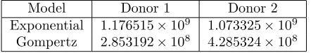
Table 2: OLS cost values for fitting the exponential (11) and Gompertz (12) to the CFSE decay data from two donors of Table 1. We see a very clear reduction in cost when using the Gompertz model.

model refinement is warranted. However, it is not possible to uniquely identify the parameterxa in either of the two models using an ordinary least squares procedure with only the data from Table 1. On the other hand, the parameterxa appears in other parts of the model (10), and it seems possible to conclude that this parameter would be readily identifiable once incorporated into (10) with the full proliferation data.

In order to at least begin to compare these two models, we set the parameter xa to the physiologically reasonable value of 50 in both models. (Values reported in the literature ranged from 10 to 100 [48, Figure 1], [50, Figure 2] and [56, Figure 3].) An ordinary least squares (OLS) procedure is then used to fit the remaining parameters (c and x(0) for the Exponential model, c, k and x(0) for the Gompertz model) for data from both donors. The results for the exponential model are shown in Figure 4 and the results for the Gompertz model are shown in Figure 5. Based upon the lines of best fit in comparison with the data, it seems clear that the Gompertz decay model more accurately describes the available data. This is confirmed by the comparison of cost given in Table 2.

(13)

0 20 40 60 80 100 120 140 160 1.5

2 2.5 3 3.5 4 4.5

5x 10

4 Donor 1 Gompertz Fit,

Time (hrs)

CFSE Intensity

0 20 40 60 80 100 120 140 160 −5000

0 5000

Donor 1 Gompertz Fit Residuals

Time (hrs)

CFSE Intensity

0 20 40 60 80 100 120 140 160 1.5

2 2.5 3 3.5 4 4.5

5x 10

4 Donor 2 Gompertz Fit

Time (hrs)

CFSE Intensity

0 20 40 60 80 100 120 140 160 −5000

0 5000

Donor 2 Gompertz Fit Residuals

Time (hrs)

CFSE Intensity

(14)

to divide. Thus we would expect slightly different parameter estimates when either of these models is used with proliferation assay data. Moreover, because this additional hour of preparation time occurs during the first hour after staining, the rapid decay observed in both data sets in Figure 3 may be partially removed from the data. Because of these considerations, it is unclear exactly how much improvement to expect from using (14) as opposed to (13) in (10).

We also remark that the primary reason for the failure of the exponential model is the location of the equilibrium point in the data (as compared to that predicted by the model). We see from Equation (11) that the exponential model predicts x→xa ast → ∞. However, it is known that CFSE stained cells retain detectable fluorescence for up to several weeks in vivo [50]. The exponential model cannot accurately account for both the rapid decline in CFSE FI during the first few hours of staining and the slow decline once the label has been stably incorporated. (We can, for the current data sets, allowxa to attain values of approximately 2.2×104; in this case the exponential model fits the data at least as well as the Gompertz model. However, this is not a physiologically reasonable value ofxa.)

Physiologically , it is known that after the conversion of CFDA-SE to CFSE by intracellular esterases, CFSE can still exit the cell at a slow rate (compared to free diffusion). However, the succinimidyl group of CFSE reacts covalently with amines attached to intracellular proteins. While some of the resulting conjugates are short-lived (either because they exit the cell or are rapidly degraded) other conjugates are stably incorporated inside the cell and remain so for an extended period of time. These stable conjugates are decreased further only by the natural turnover of the intracellular proteins to which they are bound [54]. These processes combine to produce the commonly observed “biphasic decay” of CFSE FI over time [51, 66]. In other words, it seems necessary for the rate of CFSE FI (exponential) decay to decrease in time. This is precisely the feature of the Gompertz decay model [40].

4 Parameter Estimation Procedure

With the primary features of the revised model now addressed, we are ready to validate the model with data. The current model, accounting for CFSE AutoFI and the Gompertz decay of the label, is

∂n(t, x)

∂t − ce

−kt∂[(x−xa)n(t, x)]

∂x = (15)

− (α(t, x) +β(t, x))n(t, x) +χ[xa,x∗_]4α(t,2x−xa)n(t,2x−xa).

At the right boundary (x= xmax), we expect that there are no cells which can drift (via label loss) into the computational domain. At the left boundary, a zero flux condition is imposed to prevent cells from drifting to CFSE FI values less than the AutoFI of unlabeled cells. Thus the boundary conditions are

n(t, xmax) = 0 (16)

v(t, xa)n(t, xa) = 0.

Note from (14) we havev(t, xa) = 0 for allt, and hence the left boundary condition is trivially satisfied. Finally, we assume we are given some initial condition

n(0, x) = Φ(x), (17)

which is the initial distribution of cells as a function of FI.

4.1 Model Change of Variables

While the model (15) and its associated initial and boundary conditions suitably describe the dynamics for a CFSE labeled population of dividing lymphocytes, the model is not conducive to finite difference methods for numerical solutions. The CFL condition for stability requires

∆t < ∆x

max|v(t, x)| =

∆x

maxc(x−xa)

(15)

Becausexmax>> xa, the computational domain is quite large, and max(x−xa)∼10000. Moreover, this large domain must have a relatively fine mesh, as features of the solution become less distinguishable with increasing division number. We see that, givenc∼0.1,k∼0.001, and ∆x∼0.1 (all reasonable parameters), it would take upward of 105 _{time steps to compute the solution out to} _t _{= 120 hours, and this must be done for 10}5 _points

on the structure variable grid. Rather than attempt these expensive computations, we seek a change of variables that will lead to a faster numerical solution.

The most immediate choice is to use the change of variablesz= log10x, as the data is given in this coordinate.

While this change of variables was effective in [13, 47], it is less effective here because of the different form of the label loss rate function. Instead, we use the change of variablesy= log10(x−xa). Thenx= 10y+xa and

dy dx =

1

(x−xa) ln(10).

Let ˜n(t, y) = 10y_ln(10)_n₍_{t, x}₍_y_{)) = 10}y_ln(10)_n₍_t,₁₀y₊_x_{a). We remark that the factor 10}y_{ln(10) arises from the} chain rule in the integral form of (15) and is needed to conserve the total label in the population. With this change of variables the new PDE model is

∂n˜

∂t −ce

−kt ∂

∂y

˜

n(t, y) ln 10

= −(˜α(t, y) + ˜β(t, y)−ce−kt_)˜_n₍_{t, y}₎ ₍₁₉₎

+ χ(−∞,y∗]2 ˜α(t, y+ log102)˜n(t, y+ log102),

where ˜α(t, y) = α(t, x(y)), ˜β(t, y) = β(t, x(y)) and y∗ ₌ _ymax₋_log

102. The new initial condition is ˜Φ(y) =

10y_ln(10)Φ(_t,₁₀y₊_x

a). The right boundary condition follows immediately from (16) while the left boundary has been removed toy=−∞. We remark that the CFL condition for the PDE (19) is

∆t < ∆yln 10 ce−kt

which is significantly easier to satisfy.

4.2 Parameterizations of

α

and

β

We next turn our attention to the parameterizations of the functions α(t, y) and β(t, y). Because our goal is the estimation of lymphocyte division and death rates from data, we use finite-dimensional approximations of the function spaces containing α and β so that the problem is computationally tractable and theoretically sound [11, 12]. Previous work has established that division-linked changes in proliferation and death rates are an important aspect of an accurate mathematical model [42, 46]. One of the primary motivating assumptions behind the use of a PDE model for fitting CFSE data is that the dilution of CFSE dye by division allows for the structure variable (in this case,y) to be used as a surrogate for division number [13, 45, 47]. Thus division-dependent changes in proliferation and death rates are encapsulated in the structure dependence of the functions

αandβ.

While a straightforward implementation of structure dependence forαand β has proven effective, the fact that the measured FI of a cell slowly decreases in time as a result of label loss indicates that one should take care in how the correlation between division number and structure variable is considered. As discussed at greater length in [6, 13], this label loss causes such correlation to lessen significantly. Alternatively, one might consider the total FI thatwould have been measured for a cell, if that cell did not experience any label loss. Mathematically, it is shown in [6] that this is equivalent to deriving a model in terms of an ideal label which does not decay and then changing one’s frame of reference to a moving coordinate system in which the label does appear to decay (i.e., the one relative to which the data is actually taken). Similar situations frequently arise in mechanics and fluid dynamics, where discussions of Eulerian and Lagrangian formulations abound. The key argument is to identify a cell not by its current statey, but rather by the state it would have in the event it did not undergo label loss. For a cell with statey at timet, this is equivalent to finding the intersection of the y-axis with the characteristic line passing through (t, y). Given the characteristic lines

dy dt =

(16)

it follows that the cell located at (t, y) was originally located (in the absence of division) at

s(t, y) =y+ c

kln 10(1−e

−kt₎_.

It is shown in [6, 13] that the quantity s(t, y) is more strongly correlated with division number than the quantity y. Moreover, the use of this ‘translated coordinate’ for the parameterization of α and β provided a more accurate model of the observed data when compared to the simple implementation of spatial dependence. It was hypothesized that the improvement resulted from a more direct association between division number and proliferation rate. However, that analysis was done with a different label loss function, and we desire to repeat the analysis of [13] with the new model (19) and new label loss function (equivalent to (14)). Thus we consider four different parameterizations of the proliferation rate α. In Section 5, results will be reported which demonstrate the effects of these different parameterizations on the effectiveness of the model.

First, we consider the simple case thatα=α(y). Given a fixed set of nodes{yk}, we assume

α=α(y) = Kα

X

k=1

aklk(α)(y), (20)

wherelα

k(y) are piecewise linear spline functions satisfying

lα k(yj) =

1, j =k

0, j 6=k .

It is assumed thatα(0) =α(3.5) = 0. This assumption does not have a significant impact on the model as the nodes{yk} are chosen so that the proliferation rate can be varied as necessary at all values of the state variable where cells appear in the data. It does, however, add some measure of regularity to the computed proliferation rate function.

Alternatively, as discussed above, it may prove more accurate to use the translated coordinatesin order to represent the proliferation rate of cells with a particular division number. Given a fixed set of nodes {sk}, we assume

α=α(s) =α(s(t, y)) = Kα

X

k=1

akl_k(α)(s), (21)

where the functionslα

k(s) are defined as above. Again, it is assumed thatα(0) =α(3.5) = 0.

We also consider the possibility that the proliferation rate depends explicitly on time. Indeed, we see in the data in Figure 1 that there is no proliferation at least during the first 24 hours of the assay. However, by

t= 48 hours, it is clear that the population has begun to divide. Thus the assumption of time dependence seems appropriate. As above, we can still consider the proliferation rate either in terms of the state variable y or in terms of the translated coordinates, in addition to its dependence on time. Given a set of nodes{yk}as above and a set of time nodes{tm}, we parameterize

α=α(t, y) = Kα

X

k=1

M

X

m=1 akml

(α)

k (y)l

(t)

m(t), (22)

where we now assume that the splinesl(_kα)(y) andl(mt)(t) are piecewise linear in their respective variables. Again, we ensure smoothness in the forward simulation by requiring α(t,0) = α(t,3.5) = 0. It is also assumed that

α(t, y) = 0 for allt≤24 hours.

Finally, we also consider the case thatαis parameterized in time as well as the translated coordinates. Given nodes{tm} as above and nodes{sk} in the translated variable, the proliferation rate function is then

α=α(t, s) =α(t, s(t, y)) = Kα

X

k=1

M

X

m=1

akml(kα)(s)l

(t)

m(t), (23)

where we again assume the splines l_k(α)(y) and lm(t)(t) are piecewise linear. As before, it is assumed α(t,0) =

(17)

Results from [13, 45, 47] indicate that the death rate function need not be quite as complex as the proliferation rate function. After the first few generations, the death rate of cells seems to be roughly constant. There is little reason to suspect that the death rate function depends on time and we do not consider it here. As before, we consider using the state variableyand the translated coordinatesto parameterize the death rate function. Given nodes{yk}(which may be distinct from the nodes used in the estimation of the proliferation rateα), we have

β =β(y) = Kβ

X

k=1

bkl(kβ)(y). (24)

We assumeβ(y) =b1 for ally∈[0, y1] and β(y) =bKβ for ally ∈[yKβ,3.5]. Alternatively, using the translated coordinate, we have nodes{sk}and

β=β(s) =β(s(t, y)) = Kβ

X

k=1

bkl_k(β)(s) (25)

with the assumptionsβ(s) =b1for alls∈[0, s1] andβ(s) =bKβ for alls∈[sKβ,3.5].

4.3 Computational Considerations

The change of variablesy = log10(x−xa) is a parameter-dependent change of variables, technically requiring a

‘re-gridding’ of the solution each time the parameters (specificallyxa) are changed in an optimization routine for the inverse problem. Because we use a time-stepping finite-difference method to compute the forward solution for a given set of parameters, this requirement does not constitute a great computational setback. In fact, observation of (19) reveals that the parameterxa does not appear directly in the equation to be solved, only in the change of variables that gives rise to the equation. The primary issues involve the determination of the initial condition from the data, and the comparison of the computed model solution to the data.

4.3.1 Formation of the Initial Condition

As discussed in Section 2, the cytometry data is reported as a time-series of histograms showing the numbers of cells counted into a given bin corresponding to a particular range of log CFSE FI values. That is, the histogram measures cells in thez= log10xcoordinate. While it is, in general, possible for the experimenter to set the bins

to his/her own liking, we again recall that the current data set was obtained with bins already set. The original data set, as used in [13], was taken at 24 hour intervals over the course of 6 days. Data from Day 0 (t= 0 hours) is used to form the initial condition for the model in the manner described below; the remaining data is used to fit the model to the data. At time ti, the data is stored as a set of ordered pairs (zij, n

j

i), j = 1, . . . , J(i) (the notation is meant to emphasize that the bins change each day). This ordered pair corresponds to the number of cells nj_i counted into the bin with left boundaryz_ij. (As a consequence, notice that we are unable to determine the width of the right-most bin at each time point; these points are simply removed from the data set).

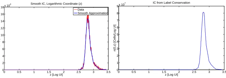
Using the data taken att = 0, we drew a smooth line through the data; ordered pairs representing the line were then determined using DataThief [63]. These smoothed histogram curves were then scaled upward into a smooth initial condition density ˆΦ(z) so that the total label content is the same for the smooth density as for the original histogram data. The results are depicted in Figure 6. Finally, given the initial condition ˆΦ(z), we transform this into an initial condition for ˜n(t, y) by noting thaty= log10(10z−xa) and using the label-preserving

identity

ˆ

Φ(z) = 10 z

10z₋_x a

˜

Φ(y(z)). (26)

This, then, provides an initial condition for (19).

4.3.2 Comparison of the Model to the Data

(18)

0 0.5 1 1.5 2 2.5 3 3.5 0

2 4 6 8 10 12 14 16 18x 10

4 Smooth IC, Logarithmic Coordinate (z)

z [Log UI]

n(0,z) [Counts]

Data

Smooth Approximation

0 0.5 1 1.5 2 2.5 3 3.5 0

1 2 3 4 5 6 7 8 9x 10

7 IC from Label Conservation

z [Log UI]

n(0,z) [Cells/Log UI]

Figure 6: Left: Smoothed histogram data att= 0 in the z coordinate. Right: Density function computed from the smoothed histogram data.

First, we must transform the structured density ˜n(t, y) into a function of z. This is done analogously to the transformation (26) above. Second, we must transform this structured density into histogram numbers. To do this, we note that at timeti, the total number of cells with FI betweenzj_i andzj_i+1 is

I[ˆn](ti, zj)≡

Z zji+1

zj_i ˆ

n(ti, z)dz≈

"

ˆ

n(ti, zij+1) + ˆn(ti, zij+1) 2

#

zji+1−z j i

, (27)

where the trapezoid rule has been used to approximate the integral. In general, we find that this is an effective method of obtaining histogram counts from the smooth density model solution. However, the varying sizes of the bins used to record the available data set poses somewhat of a problem. While the bins are generally regularly spaced, there are a few bins randomly placed in the data which are either much larger or much smaller than the neighboring bins. As a result, the histogram dataI[ˆn](ti, zj) computed from the smooth densities exhibits large jumps up or down at these points. This is strictly the result of the irregular bin sizes present in the data set and not the model solution itself. These jumps are problematic for the OLS procedure discussed below and as such these bins are removed from the data set. We emphasize again that, in future data sets, the bins can be set as needed, rather than being fixed in advance.

4.3.3 Finite Difference Computations

While (19) is defined on an infinite domain, all cells in the population maintain FI sufficiently greater thanxa, so that it is acceptable to solve (19) only on the domainy ∈[0, ymax]. In practice, we setymax independent of the parameterxa and thus solve the equation (19) on the same computational domain regardless of the parameters (i.e., those passed in by the nonlinear optimization solver). Once the solutionn(t, y) is computed, it is possible to use (26) again to change variables back to ˆn(t, z) for comparison to the data.

For the current data set, we use 512 evenly spaced nodes in the intervaly ∈[0,3.5]. The forward solution is computed using a publicly available hyperbolic PDE solver written by L. Shampine which implements the Lax-Wendroff scheme.

4.4 Ordinary Least Squares Framework

Given the appropriate parameterizations ofαandβ, we now have a complete set of parametersθ= (xa, c, k,{a},{b}) which define the model solutions. Thus in the analysis below we think of the parameterized model ˜n(t, y;θ) sat-isfying (19) given parameter θ. We now turn our attention to an inverse problem procedure which seeks to determine the parameters best describing the available data.

(19)

Parameter Minimum Maximum Units

ai 0 1 hr−1

bi 0 1 hr−1

xa 0 100 UI

c 0 0.1 UI/hr

k 0 0.005 hr−1

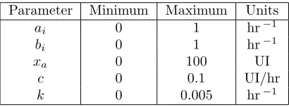
Table 3: Summary of parametersθ = (xa, c, k,{a},{b}) which define the model solution, with minimum values, maximum values, and units. Forward simulations of the model demonstrate the reasonableness of the bounds provided.

of some amount of noise. Thus, we can consider the data as a random variable

N_ij=I[ˆn](ti, zj;θ0) +Eij, (28)

where{Eij}are random variables withE[Eij] = 0 andV ar(Eij) =σ2. We remark that the assumption of constant variance for the error terms is standard for OLS formulations of inverse problems. One can examine the accuracy of such an assumption ex post facto through the use of residual-based statistical tests [7, 14, 58]. In [13], such an analysis revealed that the actual error variance was neither constant nor proportional to the square of the model solution (a ‘relative error model’). For the moment, we remark that the OLS assumption of constant variance, while possibly not exactly correct and hence not adequate for use in asymptotic parameter distributional analysis, is sufficient to provide a basis for computational parameter estimation, which will demonstrate the ability of the current model to fit the available data set. Given our uncertainty regarding the exact nature of the observed error process, we postpone a more detailed analysis of uncertainty in the estimated parameters (standard errors, confidence intervals, etc.) [7] for future work that will entail further experimental measurement error analysis and characterization.

Given the statistical model (28), we can write the data as realizations

nj_i =I[ˆn](ti, zj;θ0) +ǫij (29)

of the random variables (28). The goal of the OLS procedure is the determination of the parameter θ which minimizes the sum of squared residuals. Given the random variablesN_ij from (28), the OLS estimator is

θOLS= arg min θ∈Θ

I

X

i=1

J(i) X

j=1

(I[ˆn](ti, zj;θ)−N_ij)2= arg minJ(θ), (30)

where Θ is a set of admissible parameters for the model (see Table 3). As the data nj_i are realizations of the random variablesN_ij, it follows that the OLS estimate

ˆ

θOLS= arg min θ∈Θ

I

X

i=1

J(i) X

j=1

(I[ˆn](ti, zj;θ)−nji)2= arg minJ(θ), (31)

is a realization of the OLS estimatorθOLS. This optimization was carried out with the MATLAB constrained optimization routine fmincon_{, which implements the BFGS algorithm at each step to solve a quadratic}

sub-problem. Because such routines can become trapped in local minima, several initial iterates were tried for each optimization.

5 Results

(20)

Division Number z-axis Range 7 Nodes 13 Nodes 25 Nodes 6 [0.00,1.05] 0.0016 0.0015 0.0016 5 [1.05,1.30] 0.0043 0.0050 0.0052 4 [1.30,1.60] 0.0094 0.0103 0.0108 3 [1.60,1.90] 0.0166 0.0174 0.0206 2 [1.90,2.25] 0.0325 0.0308 0.0314 1 [2.25,2.55] 0.0284 0.0198 0.0266 0 [2.55,3.50] 0.0047 0.0097 0.0072

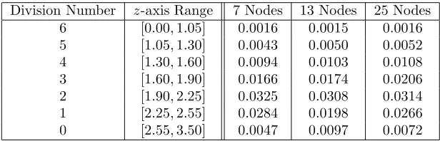
Table 4: Average proliferation rates (in units 1/hr) in terms of numbers of divisions undergone, computed from Figure 7. Using Figure 1, approximate ranges (in the coordinatez) corresponding to particular division numbers are determined. These are then used to compute the corresponding ranges in the variabley using the estimated level of cellular autofluorescence. In spite of the differences in the numbers of nodes used in the parameterization of the proliferation rate functionα(y), average proliferation values are estimated consistently for each generation.

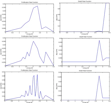
estimated proliferation and death rate functions given three different choices of nodes {yk}. First, seven nodes were evenly spaced in the interval [1.125,2.925]. Next the number of nodes was increased to 13 so that the separation between nodes was halved (and so that the increase in parameters is a refinement to the model). This procedure was repeated and the estimation was performed a third time with 25 nodes. Intuitively, each refinement must provide a more accurate fit of the model to the data, as the total OLS cost cannot increase as the number of parameters is increased. However, we also see in Figure 7 that as the number of nodes increases, the estimated proliferation rate function becomes less regular. Conversely, we see that some measure of regularity can be imposed on the function α(y) by choosing the proper set of nodes with which to estimate it (a so-called ‘regularization by discretization’ [10, 11]). While we do have available residual-sum-of-squares based statistical tests [7, 8, 14] to quantify the improvement in the model with each refinement, we choose to balance this additional information with a desire to estimate a semi-regular functionα.

It is worth remarking further that the increasingly complex structure of the function α(y) (as the number of nodes is increased) is only a relic of the estimation procedure and has nothing to do with any meaningful information regarding the population of cells being studied. In order to verify this, in Table 4 we present, for each parameterization of the function α(y) discussed in the previous paragraph, the average value of the estimated proliferation rate in terms of the numbers of divisions the cells have undergone. To compute these values, Figure 1 is used to determine approximate ranges (in the coordinatez) corresponding to each generation of cells. By changing these ranges from the variable z to y (in which the estimation of the proliferation rate function was performed), the average value of the proliferation rate function can be determined in each range. As seen in Table 4, the estimates are reasonably consistent regardless of the number of nodes used in the estimation.

Given the above discussion, we choose 13 nodes for the estimation of the proliferation rate functionα(y) and 5 nodes for the estimation of the death rate functionβ(y) in an effort maximize the flexibility of the estimation while also maintaining some regularity in the estimated functions. The OLS best-fit solution is shown in Figure 8. The optimal proliferation and death rate functions are shown graphically in the center panels of Figure 7, with numerical values provided in Tables 5 and 6. The total OLS cost for the estimation isJ(ˆθOLS) = 1.7270×1012_,

withxa = 8.2316,c= 5.6169×10−3, and k= 1.1203×10−8.

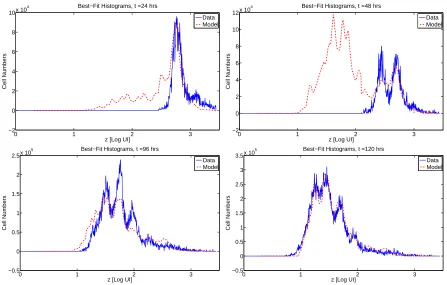
We observe that, while the OLS best-fit solution for time-independent proliferation is accurate for t = 96 and 120 hours, the model predicts far too many cells with high generation number att= 24 and 48 hours. This seems to be a manifestation of the absence of a delay (in the form of time dependence) between the time cells are stimulated and the time at which those stimulated cells divide. Thus, in addition to the arguments of Section 4.2, we have a mathematical rationale for the incorporation of time dependence into the proliferation rate. While the model does not accurately count the numbers of cells in the earlier time points, we do remark that the Gompertz label loss model and the incorporation of cellular AutoFI do accurately predict thelocation(along the horizontal axis) of the subsequent generations of cells in culture. Thus, it appears safe to conclude that the parameter γ

from [13, 47] has been effectively removed from any modeling needs.

(21)

0 0.5 1 1.5 2 2.5 3 3.5 0 0.005 0.01 0.015 0.02 0.025 0.03 0.035 0.04

Proliferation Rate Function

y [Log UI]

α

(y) [1/hr]

0 0.5 1 1.5 2 2.5 3 3.5 0 0.2 0.4 0.6 0.8 1

Death Rate Function

y [Log UI]

β

(y) [1/hr]

0 0.5 1 1.5 2 2.5 3 3.5 0 0.005 0.01 0.015 0.02 0.025 0.03 0.035 0.04

y [Log UI]

α

(y) [1/hr]

0 0.5 1 1.5 2 2.5 3 3.5 −0.005 0 0.005 0.01 0.015 0.02 0.025 0.03

Death Rate Function

y [Log UI]

β

(y) [1/hr]

0 0.5 1 1.5 2 2.5 3 3.5 0 0.01 0.02 0.03 0.04 0.05 0.06 0.07

y [Log UI]

α

(y) [1/hr]

0 0.5 1 1.5 2 2.5 3 3.5 0 0.005 0.01 0.015 0.02 0.025 0.03

Death Rate Function

y [Log UI]

β

(y) [1/hr]

(22)

0 1 2 3 −2

0 2 4 6 8 10x 10

4 Best−Fit Histograms, t =24 hrs

z [Log UI]

Cell Numbers

Data Model

0 1 2 3

−2 0 2 4 6 8 10 12x 10

z [Log UI]

Cell Numbers

Data Model

0 1 2 3

−0.5 0 0.5 1 1.5 2 2.5x 10

z [Log UI]

Cell Numbers

Data Model

0 1 2 3

−0.5 0 0.5 1 1.5 2 2.5 3 3.5x 10

z [Log UI]

Cell Numbers

Data Model

Figure 8: OLS best-fit solution withα=α(y) (13 nodes),β=β(y) (5 nodes). 21 total parameters in the model, total costJ(ˆθOLS) = 1.7270×1012_{. While the model clearly is not accurate in allowing far too many cells with}

large division number too early in time, the locations of the division peaks along the horizontal axis are quite accurate, in support of the role of autofluorescence as well as the Gompertz decay of label.

y(_kα) ak 1.1250 0.0073 1.2750 0.0123 1.4250 0.0097 1.5750 0.0196 1.7250 0.0136 1.8750 0.0262 2.0250 0.0353 2.1750 0.0301 2.3250 0.0247 2.4750 0.0137 2.6250 0.0084 2.7750 0.0034 2.9250 0.0199

(23)

y_k(β) bk 2.0000 0.0000 2.5000 0.0000 2.7500 0.0278 3.0000 0.0017 3.2500 0.0051

Table 6: Results for the OLS estimation of β(y) with 5 nodes when α=α(y) is estimated with 13 nodes. This estimated death rate function is shown graphically in the right-center panel of Figure 7.

the resulting improvement in the fit of the model to data while also accounting for the increased complexity of the model. Thus, we use the same 13 nodes as above for the structural discretization of α. For the time discretization, nodes {tm} = [48,60,72,96,120] are used. The death rate function β(y) is estimated exactly as before. This parameterization results in a model with 73 parameters. After calibration to the data, the resulting cost isJ(ˆθOLS) = 3.1302×1011_with_x

a = 6.2698,c= 4.8123×10−3, andk= 9.8091×10−8; the fit of the model to the data is shown in Figure 9. It is clear from the figure that the improvement in fitting the model to the data is quite significant. Moreover, because the inclusion of time-dependence is a refinement of the time-independent model, residual-sum-of-squares-based statistical tests exist to quantify whether the increase in complexity of the model (from 21 to 73 parameters) is justified by the resulting reduction in cost. Using the method described in [14, Ch. 3], we find that the time-independent model can be rejected in favor of time-dependent proliferation with very high (>99.999%) confidence.

Thus we see that, once the proliferation rate is allowed to vary as a function of time, the model very closely mimics the data in terms of the numbers of cells in each generation at a given time. Moreover, we again point out that the physiological explanation for the the dilution of FI by division, as well as the Gompertz model for natural FI decay do an excellent job of predicting the locations (along the horizontal axis) of each generation of cells. Still, we continue further to consider one more potential improvement to the model. Following the analysis of [13] and the discussion of Section 4.2, we consider parameterizing the proliferation and death rate functions in terms of the ‘translated coordinate’s. As discussed previously, it is expected that this coordinate correlates much more closely with division number than the coordinateszory. As such, estimation of the proliferation and death rates in terms of this quantity should provide a more meaningful (and less biased) estimate when these estimated functions are analyzed in terms of division number (in the manner of Table 4). It is worth noting the parameterization of the functionsαandβ in terms ofsis not a model refinement (compared to parameterization in terms ofy) so that the model comparison tests described above are not directly applicable. While additional (e.g. information-theoretic) tests could be used, we forgo that analysis here in the interest of brevity. However, as will be shown, parameterization in terms ofsdoes in fact provide a more meaningful correlation between the estimated cell turnover rates and division number (in additional to providing a slightly lower cost!), which justifies its use.

The nodes used from the proliferation and death rate functions, as well as the estimated rates at those nodes, are given in Tables 7 and 8, respectively, and the functions are shown graphically in Figure 10. As before, 73 parameters arise in this parameterization of the model. The total cost is J(ˆθOLS) = 3.0901×1011_{, with} xa = 6.4053,c= 5.5246×10−3, andk= 5.0323×10−4; the fit of the model to the data is shown in Figure 11.

Visually, the fit of this model (usingsfor the structure discretization of the proliferation and death rates) is comparable to the previous model (usingy), and the cost is slightly lower. The significant advantage in usings, as noted above, is that the translated coordinatesis more strongly correlated with division number. To see this, the data from Figure 1 are shown in the translated coordinate in Figure 12. While there is still some overlap among the generations of cells in the histogram data, the translated coordinate provides an axis on which cells do not drift as they slowly lose CFSE FI. Particularly when compared to Figure 1, we see that it is much easier to assign distinct regions of thesaxis to particular division numbers when compared to using thez(and thusy) axis. Moreover, because cells do not drift to the left on thesaxis, regions assigned to particular division numbers remain valid for all time.

(24)

0 1 2 3 −2

0 2 4 6 8 10x 10

z [Log UI]

Cell Numbers

Data Model

0 1 2 3

−2 0 2 4 6 8 10x 10

z [Log UI]

Cell Numbers

Data Model

0 1 2 3

−0.5 0 0.5 1 1.5 2 2.5x 10

z [Log UI]

Cell Numbers

Data Model

0 1 2 3

−0.5 0 0.5 1 1.5 2 2.5 3 3.5x 10

z [Log UI]

Cell Numbers

Data Model

Figure 9: OLS best-fit solution with α = α(t, y), β = β(y). 73 total parameters in the model, total cost

J(ˆθOLS) = 3.1302×1011_.

tk

s(_kα) 48 60 72 96 120 1.1875 0.0713 0.1404 0.0000 0.0000 0.0167 1.3375 0.2028 0.0522 0.0001 0.0000 0.0175 1.4875 0.6036 0.0303 0.0376 0.0009 0.0281 1.6375 0.2896 0.0138 0.0004 0.0075 0.0251 1.7875 0.0618 0.0001 0.0000 0.0409 0.0220 1.9375 0.0091 0.0345 0.0020 0.0119 0.0220 2.0875 0.0837 0.0002 0.0400 0.0326 0.0391 2.2375 0.0018 0.1956 0.0083 0.0001 0.0231 2.3875 0.0050 0.0059 0.0962 0.0394 0.0463 2.5375 0.0000 0.1949 0.0128 0.0050 0.0000 2.6875 0.0155 0.1101 0.1528 0.0422 0.0239 2.8375 0.0351 0.0446 0.0000 0.0000 0.0000 2.9875 0.0346 0.0000 0.0012 0.1317 0.0092

(25)

s(_kβ) bk 2.0000 0.0054 2.5000 0.0000 2.7500 0.0238 3.0000 0.0061 3.2500 0.0000

Table 8: Results for the OLS estimation ofβ(s) when α=α(t, s). This estimated death rate function is shown graphically in Figure 10

0 0.5 1 1.5 2 2.5 3 3.5 0 50

100

0 0.2 0.4 0.6

t [hr] s [Log UI]

α

(t,s) [1/hr]

0 0.5 1 1.5 2 2.5 3 3.5

0 0.005 0.01 0.015 0.02 0.025

Death Rate Function