Development of Tensor Network Algorithms for Studying Classical and Quantum Many Body Systems

(1)

Classical and Quantum Many-Body Systems

Thesis by

Matthew Theodore Fishman

In Partial Fulfillment of the Requirements for the Degree of

Doctor of Philosophy

CALIFORNIA INSTITUTE OF TECHNOLOGY Pasadena, California

2018

(2)

Matthew Theodore Fishman

(3)

ACKNOWLEDGEMENTS

First and foremost I would like to thank my parents, without whom none of this would be possible. Their commitment to my success in life is unwavering, and I owe them for everything I have.

Of course I would like to thank my advisors, Steve White and John Preskill, as well as the other members of my committee, Garnet Chan and Lesik Motrunich.

Steve took me under his wing when I was looking for research guidance. His kindness, generosity and patience are unmatched, and he has always been available to talk and to give insight and advice for any problem I might have. It was a great privilege and honor to work with him and observe his scientific process. He is able to pinpoint the exact source of a problem and immediately propose a clever and original solution. Working with and talking to him has been humbling, and has shaped the way I approach problems I encounter.

John creates an environment in his group for exploration, and this work would not have been possible without the freedom he allowed. It was inspiring to see the wide range of problems members of his group work on, and the surprising range of technical topics with which John could engage. John is known for asking deep and insightful questions on research topics that are not directly in his area of expertise, and his reputation preceded him. Throughout my PhD I had a small voice in the back of my head with questions John might ask me about my research, and that was a guiding force for me to ask deeper questions or change research directions.

I am grateful to Garnet for encouraging me to talk to Steve early on in my PhD. Garnet is an incredibly ambitious and energetic scientist, and it has been great to get to discuss research with him over the years.

(4)

I would particularly like to thank Glen Evenbly, who as a postdoc at Caltech in John’s group introduced me to this field of research as well as to Steve. Glen approaches the messy world of computational physics with an unmatched clarity and care, and I can only hope to approach problems with his level of precision. While he was at Caltech and afterward as a postdoc at UCI with Steve, most of the research ideas I had passed by him, and I quickly learned to treat his answers to questions I had as the ultimate authority on the topic.

I am indebted to Micheal Beverland, a former graduate student of John’s who convinced me to speak to Glen when I was looking for topics of research. His friendship and guidance throughout my PhD helped get me through some of my most difficult times here. He is wise beyond his years, and one of the most thoughtful people I have ever met. I would also like to thank Sam Johnson for her friendship and support when I was starting out here at Caltech.

I would like to thank Frank’s students including but not limited to Valentin Stauber, Burak Sahinoglu, Matthias Bal, Laurens Vanderstraeten, etc. for their friendship and scientific collaborations while I was visiting them in Europe. I would also like to thank all of my friends in Austria and Belgium, who made me feel at home when I was away from my friends and family.

It was a privilege to have the opportunity to engage with so many scientists at Caltech, UCI, and elsewhere, such as Miles Stoudenmire, Mike Zaletel, Martin Ganahl, Ashley Milsted, Julian Rincon, Philippe Corboz, Chris White, Brenden Roberts, Guifre Vidal, Zhenyue Zhu, Chia-Min Chung, Thomas Baker, etc. I have found that the scientists in this field of research are passionate, curious and supportive, and I appreciate the chance I have had to get to interact with them.

(5)

ABSTRACT

The field of tensor networks, kicked off in 1992 by Steve White’s invention of the spectacularly successful density matrix renormalization group (DMRG) algorithm, has exploded in popularity in recent years. Tensor networks are poised to play a role in helping us solve some of the greatest open physics problems of our time, such as understanding the nature of high-temperature superconductivity and illuminating a theory of quantum gravity. DMRG and extensions based on a class of variational states known as tensor network states have been indispensable tools in helping us understand both numerically and theoretically the properties of complicated classical and quantum many-body systems. However, practical challenges to these techniques still remain, and algorithmic developments are needed before tensor network algorithms can be applied to more physics problems. In this thesis we present a variety of recent advancements to tensor network algorithms.

First we describe a DMRG-like algorithm for noninteracting fermions. Noninter-acting fermions, naturally being gapless and therefore having high levels of entan-glement, are actually a challenging setting for standard DMRG algorithms, and we believe this new algorithm can help with tensor network calculations in that setting.

Next we explain a new algorithm called the variational uniform matrix product state (VUMPS) algorithm that is a DMRG-like algorithm that works directly in the thermodynamic limit, improving upon currently available MPS-based methods for studying infinite 1D and quasi-1D quantum many-body systems.

(6)

(7)

PUBLISHED CONTENT AND CONTRIBUTIONS

1_{M. T. Fishman and S. R. White, “Compression of correlation matrices and an}

efficient method for forming matrix product states of fermionic gaussian states”, Phys. Rev. B92, 075132 (2015).

2_{V. Zauner-Stauber, L. Vanderstraeten, M. T. Fishman, F. Verstraete, and J.}

Haege-man, “Variational optimization algorithms for uniform matrix product states”, Phys. Rev. B97, 045145 (2018).

3_{M. T. Fishman, L. Vanderstraeten, V. Zauner-Stauber, J. Haegeman, and F.}

Verstraete, “Faster Methods for Contracting Infinite 2D Tensor Networks”, arXiv:1711.05881.

Chapter2is based on work published with Steve White in Ref. [1]. The work was initiated by the insight from Steve to diagonalize a correlation matrix with a local set of unitary gates and his idea that a discrete orthogonal wavelet transformation can be seen as a single-particle MERA. I was the main contributor (I performed all of the calculations, developed the technique to form a many-body MPS from the single-particle gates, developed the technique to produce a free fermion MERA, and developed the DMRG-like algorithm for obtaining the free fermion MPS from a quadratic Hamiltonian).

Chapter3 is adapted from work published with Valentin Zauner-Stauber, Laurens Vanderstraeten, Frank Verstraete, and Jutho Haegeman in Ref. [2], of which I was a minor contributor. The chapter focuses on parts of the algorithm proposed in that reference that I contributed most to (helping to determine the preferred technique for obtaining the uMPS from the zero-site and one-site wavefunctions and the parallel algorithm for extending to multi-site unit cells).

Chapter4is primarily my own work. Some of it appears in Ref. [3] (posted to the arXiv and accepted for publication in Phys. Rev. B). I wrote the review of currently available CTMRG methods as well as developed the new CTMRG algorithm for contracting asymmetric tensor networks. Jutho pointed out the simplified version of the CTMRG method of Corboz et al.

(8)

(9)

LIST OF FIGURES

21 Fig. 21(a) shows the occupationsnband corresponding entanglement

S1(nb) from diagonalizing a block of B = 16 sites in the middle of a system of free gapless fermions on N = 1000 sites at half filling. The minimum and maximum eigenvalues, n1and n16, differ from 0 and 1 by≈1.74×10−11. The eigenvalues closest to 1/2, 1/2−n8 =

n9 − 1/2 ≈ 0.21, have entropies S1(n8) = S1(n9) ≈ 0.60, which are close to the maximum of S1(1/2) = log(2) ≈ 0.69. Fig. 24(b) shows examples of eigenvectors from the same diagonalization. The eigenvectors with eigenvalues near 0 and 1, which contribute very little to the entanglement, are localized in the middle of the block, while the eigenvectors with eigenvalues closer to 1/2 which contribute most to the entanglement have large support on the edges of the block. 8 24 In Fig. 24(a) we show schematically the procedure to obtain, given

an approximate eigenvector ®vof the correlation matrix Λ, the set of local rotation gates that make up our compressed correlation matrix. The example shown is for a block size B = 4 and system size N =

8. Fig. 24(b) shows that, by conjugating the correlation matrix by the gates obtained, the correlation matrix is approximately partially diagonalized. . . 13 25 Fig. 25(a) shows the overall gate structure obtained by the

(12)

26 An example of an alternative diagonalization scheme resulting in a MERA-like gate structure. Here we show a section of the first two renormalization steps, with 12 sites shown in the first layer and 6 renormalized sites shown in the second. A block size of B = 4 is used. For this block size there are two layers of disentanglers and one layer of isometries per level of the MERA. Open legs at the top of each layer correspond to diagonal modes of the correlation matrix (with eigenvalues 0 or 1) and are ignored at the next layer. . . 16 27 Here we show an example of a discrete wavelet transform written in

the gate notation introduced in this paper. We show the D4 wavelet, which corresponds to a fermionic Gaussian MERA with one layer of disentanglers and one layer of isometries per layer. w1 and s1 (w2 and s2) label wavelet and scaling functions for the first (second) layer. Taking θ1 = π/6 and θ2 = 5π/12, we reproduce the conventional scaling coefficients for the D4 WT,a®T =(a1,a2,a3,a4)=(1+

√ 3,3+ √

3,3−√3,1−√3)/(4√2). . . 18 28 Here we show explicitly how to obtain the scaling and wavelet

coefficients of the D4 WT from the circuit construction. Taking θ1 = π/6 and θ2 = 5π/12, in (a) and (b) we reproduce the con-ventional scaling coefficients for the D4 WT, a®T = (a1,a2,a3,a4) = (1+√3,3+√3,3−√3,1−√3)/(4√2), up to a trivial reversal in the order. In (c) with the same choice of angles we reproduce the con-ventional wavelet coefficients(a4,−a3,a2,−a1), again up to a trivial reversal and sign. . . 19 212 Examples of occupied and unoccupied modes found in the

diagonal-ization process. Fig. 212(a) shows occupied/unoccupied modes for δ= 0.4 (energy gap≈ 0.806135t). Fig. 212(b) shows occupied/unoc-cupied modes forδ =0 (energy gap≈0.146088). . . 24 213 Examples of deviations in occupations at the end of the

(13)

214 Block size B needed for a relative error in the energy of < 10−6 as a function of number of sites N for spinless, gapless fermions with open boundary conditions at half filling. As expected from arguments about the entanglement of a critical system, we find B ∼ log(N), tested up to N = 216 =65536 sites (note the log scale on the x axis). To study systems of this size and avoid theO(N3)diagonalization of the hopping Hamiltonian, we obtain the correlation matrix using the GDMRG algorithm as explained in Appendix 2.B. . . 26 215 Relative error in the energy for the proposed GMERA construction

for increasing number of sites for a block size B = 10. The system analyzed is the ground state of free fermions hopping on a lattice with open boundary conditions. All errors are below 10−6. As expected for a MERA, the error is seen to saturate for large N, indicating a fixed block size is sufficient to obtain an accuracy <10−6up to very large system sizes. . . 27 216 A plot of the time to form the MPS approximation of gapped and

gapless free fermion ground states at half filling as a function of sites

N using gates from a GMPS. The bond dimensions are chosen large enough such that the relative errors in the energy of the MPS are below 10−6. The block size of the GMPS used to form the MPS are the minimum required to obtain a GMPS with a relative error in the energy of 10−6. A cutoff in the singular values of the SVD of 10−11 was used when applying the gates to form the MPS using the method described in Section 2.3.4. For the gapped case, the SSH model with δ = 0.1 is used, corresponding to an energy gap of ∆≈ 0.2t (exact as N → ∞). . . 28 4.41 Plots comparing our new method for obtaining the CTMRG projector

(14)

5.41 Plots of the error in the magnetization for the isotropic 2D classical Ising model at two temperatures near criticality, where (b) is closer to criticality than (a). The network has a bond dimension of d = 2, and a boundary MPS bond dimension of χ = 600 is used. A fully symmetric CTM ansatz is used for CTMRG and the FPCM, and full symmetry is exploited in VUMPS. The speedup of VUMPS and the corner method over CTMRG increases as one gets closer to criticality. Stars indicate the environment tensors have reached a fixed point, and data points beyond those points are numerical fluctuations and were not shown in order to simplify the plot. . . 97 5.42 Convergence time as a function of inverse temperature above

criti-cality, β/β_c−1, for the 2D classical Ising model. For all data points, a boundary MPS bond dimension of χ = 600 is used. All data is converged to an error in the magnetization of < 2×10−9. The inset shows the ratio of the convergence time of CTMRG and VUMPS with respect to the FPCM convergence time. . . 98 5.43 Plots of error in magnetization for the isotropic ferromagnetic 2D

(15)

5.44 (a) Plot of magnetization for the 2D classical XY model, for network bond dimensiond = 25 and boundary MPS bond dimension χ= 50. (b) Plot of error in energy (compared to Monte Carlo results) for the 2D quantum Heisenberg model. The network bond dimension is

d = 25 (or PEPS bond dimension √d = 5), and the MPS boundary bond dimension χ = 100. (c) Plot of error in the norm (where the “exact" results is taken to be an extrapolation of the norm in the limit of a large environment bond dimension) of the chiral RVB PEPS. The network bond dimension isd= 9 (or PEPS bond dimension

√

(16)

C h a p t e r 1

INTRODUCTION

The field of tensor networks, kicked off in 1992 by Steve White’s invention of the spectacularly successful density matrix renormalization group (DMRG) algorithm, has exploded in popularity in recent years. Tensor networks are poised to play a role in helping us solve some of the greatest open physics problems of our time, such as understanding the nature of high-temperature superconductivity and illuminating a theory of quantum gravity. White’s DMRG algorithm is best suited for calculating ground states of gapped, one-dimensional (1D) quantum many-body systems, a setting in which it is by far the most effective tool.

Unfortunately our most interesting open physics problems are in the real world, where there is oftentimes more than one dimension and a finite temperature. Al-though it has exponential scaling when applied to dimensions higher than one, DMRG is such a reliable algorithm that it is still the tool to beat for many 2D problems. DMRG, based on a variational state known as the matrix product state (MPS), can also be generalized for direct use in higher dimensions. It has become clear since the invention of DMRG that MPSs are simply the simplest variational state of a more general class of states known as tensor network states. The most popular of these higher-dimensional formulations for practical calculations makes use of a variational class of states known as tensor product states (TPS) or projected entangled pair states (PEPS), and in terms of those states polynomial-scaling algo-rithms can be formulated for problems in two and higher dimensions. Unfortunately these generalizations of the DMRG algorithm are more challenging to work with in practice, though a lot of progress has been made over the years to turn them into competitive numerical tools.

(17)

In Chapter 2, we present on a DMRG-like algorithm for noninteracting fermions. Tensor network states can be thought of as efficient data compressions: the amount of classical information in a quantum many-body state naively scales exponentially with the number of degrees of freedom in the system. In practice, however, most physical states we would encounter appear to not contain this much information, and tensor network states can be thought of as efficient compressions of the general quantum state into a much more efficient form. We show that, even though they already have an efficient representation, noninteracting quantum many-body states can be compressed into even more efficient forms, and we present simple and intuitive algorithm for performing that compression by performing local diagonalizations of the correlation matrix. Noninteracting fermions, naturally being gapless and therefore having high levels of entanglement, are actually a challenging setting for standard DMRG algorithms, and we believe these new algorithms can help with DMRG calculations in that setting.

In Chapter3, we present on a new algorithm called the variational uniform matrix product state (VUMPS) algorithm that is a DMRG-like algorithm that works directly in the thermodynamic limit. The algorithm uses the ansatz of a uniform matrix product state (uMPS), and explicitly optimizes that variational state. This is in contrast to the infinite DMRG (iDMRG) algorithm, which is a DMRG algorithm that reaches the thermodynamic limit by growing the system size at each step, and the infinite time evolving block decimation (iTEBD) algorithm, which works with a uMPS in the thermodynamic limit but optimizing the state with a power method instead of variationally. Benchmark results presented in Ref. [2] show that this algorithm performs better than the state-of-the-art algorithms for a variety of 1D and quasi-1D systems in the thermodynamic limit, which is the exact limit of interest for many tensor network algorithms.

In Chapter4, we present a short review of the corner transfer matrix renormalization group (CTMRG) algorithm of Nishino and Okunishi. CTMRG is one way to extend DMRG for studying 2D classical statistical mechanics problems. It also in practice plays a fundamental role in the most challenging part of infinite PEPS (iPEPS) calculations. In this chapter, we also present a new CTMRG approach that improves the numerical stability for contracting asymmetric two-dimensional tensor networks compared to the most commonly used method.

(18)

(19)

C h a p t e r 2

FREE FERMION DENSITY MATRIX RENORMALIZATION

GROUP

1_{M. T. Fishman and S. R. White, “Compression of correlation matrices and an}

efficient method for forming matrix product states of fermionic gaussian states”, Phys. Rev. B92, 075132 (2015).

Here we present an efficient and numerically stable procedure for compressing a correlation matrix into a set of local unitary single-particle gates, which leads to a very efficient way of forming the matrix product state (MPS) approximation of a pure fermionic Gaussian state, such as the ground state of a quadratic Hamiltonian. The procedure involves successively diagonalizing subblocks of the correlation matrix to isolate local states which are purely occupied or unoccupied. A small number of nearest neighbor unitary gates isolates each local state. The MPS of this state is formed by applying the many-body version of these gates to a product state.

We treat the simple case of compressing the correlation matrix of spinless free fermions with definite particle number in detail, though the procedure is easily extended to fermions with spin and more general BCS states. We also present a DMRG-like algorithm to obtain the compressed correlation matrix directly from a hopping Hamiltonian. In addition, we discuss a slight variation of the procedure which leads to a simple construction of the multiscale entanglement renormalization ansatz (MERA) of a fermionic Gaussian state, and present a simple picture of orthogonal wavelet transforms in terms of the gate structure we present in this paper. As a simple demonstration we analyze the Su-Schrieffer-Heeger model (free fermions on a 1D lattice with staggered hopping amplitudes).

2.1 Introduction

(20)

uses, more efficiently compresses the wavefunction when interactions are strong, due to lower entanglement in a real-space basis.

In this paper, we introduce a new algorithm for efficiently producing an MPS representation for ground states of noninteracting fermion systems. Why is this useful, when DMRG is most useful in the opposite regime? This would be a valuable tool in a number of situations. For example, a powerful and widely used class of variational wavefunctions for strongly interacting systems begin with a mean-field fermionic wavefunction, and then one applies a Gutzwiller projection to reduce or eliminate double occupancy[7]. It could be very useful to find the overlaps of a DMRG ground state with a variety of such Gutzwiller states to help understand and classify the ground state. Once one has the MPS representation of the mean field state, the Gutzwiller projection is very easy, fast, and exact, whereas in other approaches it usually must be implemented with Monte Carlo. One might also begin a DMRG simulation with such a variational state, or in some cases with a mean field state without the Gutzwiller projection. Being able to represent fermion determinantal states as MPSs in a very efficient way also opens the door to using DMRG ground states as minus-sign constraints in determinantal quantum Monte Carlo, in particular in Zhang’s constrained path Monte Carlo (CPMC) method[8,9]. In this case one would hope that, for systems too big for accurate DMRG, at least the qualitative structure of the ground state could be captured by DMRG, and then the results could be made quantitative with the Monte Carlo method.

(21)

with an efficient method for forming the MPS of a fermionic Gaussian state. We also present a new and simpler method for obtaining a fermionic Gaussian MERA (GMERA), the MERA of a fermionic Gaussian state, as a simple extension.

Our approach to producing the MPS of a fermionic Gaussian state also produces a compressed form of the correlation matrix itself, which we call a fermionic Gaussian MPS (GMPS), which might be useful in very different contexts where the single-particle matrices are very large. This compressed form expresses the

N×N correlation matrix in terms ofO(BN)real angles which parametrize nearest neighbor rotation gates, where B N for states with low entanglement. The compressed form can be utilized directly. For example, ordinarily multiplying an arbitrary vector by the correlation matrix, which is not sparse, requiresO(N2)

operations, but by using the compressed form onlyO(BN)operations are needed. For simplicity, the algorithm we introduce first utilizes the correlation matrix as the initial input. However, in Appendix2.Bwe present a DMRG algorithm in the single particle context, which we call fermionic Gaussian DMRG (GDMRG), that starts with a single particle Hamiltonian matrix and outputs the ground state correlation matrix in compressed form as a GMPS at a greatly reduced cost compared to directly diagonalizing the Hamiltonian matrix,O(B3N)as opposed toO(N3). This algorithm exploits the close relationship between the correlation matrix and the density matrix of a many particle state, and many tensor network algorithms can similarly be translated into a single particle framework.

(22)

2.2 Background on Fermionic Gaussian States and Correlation Matrices

Consider the Hamiltonian for a 1D system of noninteracting fermions

ˆ

H =

N

Õ

i,j=1

ˆ

a_i†Hi jaˆj, (2.1)

whereaianda

†

i are fermion operators andH =[Hi j]is a Hermitian matrix (H = H

† ). We assume that the Hamiltonian terms are local (so the matrixHis band-diagonal).

Diagonalizing the matrix H, we have H = U DU† where U is unitary and D is diagonal such that Dk k0 = _kδ_{k k}0. The Hamiltonian can then be put into diagonal form,

ˆ

H =

N

Õ

k=1

kaˆ†_kaˆk, (2.2)

where the operators which create the single particle energy eigenstates are

ˆ

a†_k =

N

Õ

i=1

Uikaˆ†_i. (2.3)

Assumingk ≤ k0 ifk < k0, the ground state is

|ψ₀i=

NF Ö

k=1

ˆ

a†_k|Ωi, (2.4)

whereNF is the number of particles in the system.

Thecorrelation matrixis

Λi j =

D ˆ

a_i†aˆj

E =

NF Õ

k=1

U_ik∗Uj k. (2.5)

The correlation matrix fully characterizes|ψ₀ibecause all correlation functions, and therefore all observables, can be factorized into two-point correlators using Wick’s theorem. Note that the eigenstates ofH are also the eigenstates ofΛ(the sameU

that diagonalizesH also diagonalizesΛ). However, the eigenvalues ofΛare either 1 (occupied) or 0 (unoccupied). The massive degeneracy of Λmeans that we can make arbitrary changes of basis among the eigenstates of Λas long as we do not mix occupied and unoccupied states.

(23)

0 0.5 1.0

5 10 15

b

nb

S1(nb)

(a) Eigenvalues and entanglement entropy.

-0.5 0 0.5

495 500 505

Amplitude

of

eigen

vector

i

n1≈0

n8≈0.29

n16≈1

[image:23.612.125.501.85.233.2]

(b) Example eigenvectors.

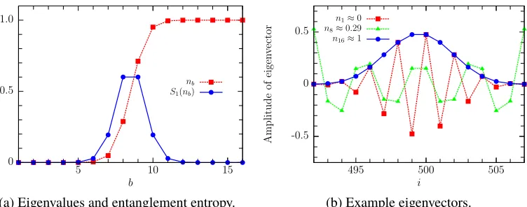
Figure 21: Fig. 21(a) shows the occupations nb and corresponding entanglement

S1(nb)from diagonalizing a block ofB = 16 sites in the middle of a system of free

gapless fermions on N = 1000 sites at half filling. The minimum and maximum eigenvalues, n1 and n16, differ from 0 and 1 by ≈ 1.74×10−11. The eigenvalues

closest to 1/2, 1/2−n8= n9−1/2≈ 0.21, have entropiesS1(n8) = S1(n9) ≈ 0.60, which are close to the maximum of S1(1/2) = log(2) ≈ 0.69. Fig. 24(b) shows

examples of eigenvectors from the same diagonalization. The eigenvectors with eigenvalues near 0 and 1, which contribute very little to the entanglement, are localized in the middle of the block, while the eigenvectors with eigenvalues closer to 1/2 which contribute most to the entanglement have large support on the edges of the block.

rotating into the basis of these eigenvectors, we can locally diagonalize the correla-tion matrix, which will lead to a compression of the state. These eigenvectors have eigenvalues near 1 or 0, which makes them (approximate) eigenvectors of the entire correlation matrix and therefore uncorrelated with the rest of the system. What makes it possible to find a localized eigenvector?

The answer is the limited entanglement structure of the states we are interested in (ground states of local Hamiltonians). Consider the entanglement entropy of our fermionic Gaussian state, which can be calculated directly from the correlation matrix. Divide the system into an arbitrary subblock Bof B sites (with the corre-sponding submatrix ofΛ, which we callΛB) and the rest of the system. We would like to know how large of a block sizeBwe need to find a localized eigenvector. If the matrixΛB has eigenvalues{nb} forb ∈ B, with 0 ≤ nb ≤ 1, the entanglement

entropy of the subblockB,SB ≡ −Tr[ρˆBlog(ρˆB)](where ˆρB is the reduced density matrix of the state in subblockB), is

SB({nb})=

Õ

b∈B

(24)

where S1 nb = nblog nb + 1 nb log 1 nb . This expression has been

shown elsewhere[12–15]. We show a simple, self-contained derivation of it in Appendix2.A. Note thatS1(nb)vanishes for bothnb→ 0 andnb→1.

The maximum amount of entanglement a block of size B can contain is when

nb = 1/2 for all b ∈ B, so SB ≤ Blog(2). This reflects a volume law

entangle-ment in the “volume" B. However, ground states of 1D local Hamiltonians have entanglement that is much smaller, either of order unity (if the system is gapped), or the entanglement grows as log(B)if the system is gapless. To avoid the volume entanglement, most of the block eigenvaluesnbmust be exponentially close to 0 or

1. In other words, as soon as we makeBbig enough so that the entanglement begins to saturate, except for a possible slow logarithmic growth, we should find at least one eigenvalue very close to 0 or 1. For gapless free fermions in 1D on N =1000 sites, we show example eigenvalues, eigenvectors, and corresponding entanglements of a block of B = 16 in the middle of the correlation matrix in Fig. 21. Even for gapless free Fermions, with a block size of onlyB = 16 we find many eigenvalues near 0 or 1 (many localized eigenvectors). We use this observation next to develop algorithms to locally diagonalize correlation matrices and in the process find a very compressed form.

2.3 Algorithms

2.3.1 Compressing a Correlation Matrix as a GMPS

We begin the procedure by diagonalizing the upper left B× B subblock of a cor-relation matrix Λ of a pure fermionic Gaussian state. Assume that the state has some local entanglement structure, for example it is the ground state of a local Hamiltonian in 1D. For now, we imagine our system has open boundary conditions. For simplifying the discussion, from here on we assume our Hamiltonian is real (and therefore symmetric and diagonalized by an orthogonal matrix). We discuss the more general complex case at the end of the section. LetBbe the group of sites 1, . . .Bon the left end of the system, andΛB be the associated subblock ofΛ. Also, let {nb} be the eigenvalues of ΛB for b ∈ B where 0 ≤ nb ≤ 1. (This constraint

on the eigenvalues of the subblock follows from the fact that bothΛand 1−Λare positive semi-definite.)

We increaseBuntil we find somenbthat is nearly 1 or 0 within a specified tolerance,

(25)

-0.5

0

0.5

5

10 Amplitude

of

mo

de

Site

nunocc≈0

[image:25.612.145.454.79.298.2]

nocc≈1

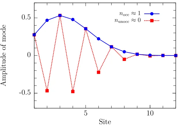
Figure 22: Examples of approximate occupied and unoccupied eigenvectors of Λ

obtained from diagonalizingΛB where subblockBare sites 1, . . . ,B. Λis formed from the ground state of ˆH = −tÍN−1

i=1 (aˆ

†

iaˆi+1+ h.c.)for N = 1024 at half filling

(NF = N/2). A block size of B = 12 is used. Eigenvectors with highest (nocc)

and lowest (nunocc) eigenvalues found from diagonalizing subblock B are shown.

We find 1− nocc = 2.4×10−15 and nunocc = 7.3× 10−16, so the occupations are accurate to nearly machine double precision. 1−nocc andnunocc should be equal at

half filling (because of particle-hole symmetry), but are different in this case as a result of roundoff errors.

the MPS we will form. In Fig. 22 we show the most occupied and unoccupied eigenvectors of ΛB for B = 12 for a system of gapless free fermions in 1D with

N =1024 sites. We see thatB=12 is sufficient to give deviations from occupancies of 0 or 1 to nearly machine double precision. The eigenvalues found in the bulk likely will not be as accurate, because states in the bulk will generally be more entangled than the ones on the edge. The smooth fall-off to zero at the right edge of the block is characteristic of these modes and is a result of diagonalizing the block on the left-most boundary of the system. The localized states we find here areleastentangled with the rest of the system. This is in contrast to the dominant Schmidt states that are utilized within DMRG which have degrees of freedom that are localized at the edge of the block.

(26)

transformation ofΛwill makeΛ₁₁ =n1, and zero out the rest of row 1 and column

1. The matrix of eigenvectors ofΛB would produce such a matrix (expanding it to

N × N by putting ones on the diagonal), but this B× B matrix does not translate well to many-particle gates to use in constructing an MPS.

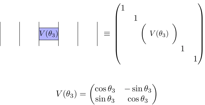
We now introduce gate/circuit diagrams which apply equally well to simple matrix manipulations ofΛandto many-particle tensor networks. The basic ingredient of the diagrams are two site nearest neighbor unitary gates. In Figure 23 we show the relation between a gate and a matrix. In a later section we show how a gate is interpreted in the many-particle context of a tensor network. We consider nearest neighbor gates because these translate to fast MPS algorithms—typically, a non-nearest neighbor gate is implemented as a set of swap gates to bring the sites together, a nearest neighbor gate, followed by swaps to return to the original ordering of the sites, which is much slower than a single nearest neighbor gate. In the special case that the intermediate sites are in product states, i.e. bond dimension 1, nonlocal gates are also inexpensive, and we use these in our MERA algorithm.

Returning to the task of moving the least entangled state ®vto the first site, a set of

B−1 two-site gates suffices. The first gate acts on sites(B−1,B), and we label it

VB−1. In general, we take

Vi =V(θi)=

cosθi −sinθi

sinθi cosθi

!

. (2.7)

We chooseθB−1=tan−1(vB/vB−1), whereviis theithcomponent of the (un)occupied

eigenvector of interest®v. With this choice,VB−1acting on®vT =

v1 . . . vB−1 vB

sets the last component, vB, to zero, and produces a new value of vB−1 → v0_B−1.

In other words, we solve for θB−1 so that v®TVB−1 =

v1 . . . vB−1 vB

VB−1 =

v1 . . . v0_B₋₁ 0

. Next we rotate sites(B−2,B−1), withθB−2= tan−1(v0_B₋₁/vB−2),

and continue in this fashion. The action of all these gates onv®T gives δi,1, so they

act to change the basis into the one containing®v.

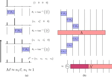
We take VB = V(θB−1)V(θB−2). . .V(θ1). This procedure is shown schematically

for a simple case in Fig. 24(a). We then apply the gates to Λ. The transformed correlation matrix V_B†ΛVB will have n1 ≈ 1 or 0 as the top left entry (and nearly

(27)

≡







1

1 





V

(

θ

3

)

V

(

θ

₃

) =

cos

θ

3

−

sin

θ

3

sin

θ

B is decreased to the remaining number of sites. After N blocks, we will have approximately diagonalizedΛ.

The overall unitary transformation isV = VB₁VB₂. . .VB_N−1. The matrixV

decom-posed into the 2×2 rotation gates{V(θi)}forN =8 andB=4 is shown in Fig.25(a).

The N ×N unitary approximately rotates our single particle basis from real space to what we refer to as theoccupation basis, which is one of the highly degenerate eigenbases of the correlation matrix. ConjugatingΛbyV gives us a matrixV†ΛV

that is nearly diagonal, with NF values on the diagonal close to 1 corresponding

to occupied modes and N − NF values on the diagonal close to 0 corresponding

to unoccupied modes. In total, the procedure as described would requireO(BN)

nearest neighbor rotations, where Bis the largest block size needed for the desired accuracy of the representation of the correlation matrix.

(28)

~vT = v1 v2 v3 v4 v1 v2 v30 0

v1 v002 0 0

1 0 0 0

V(θ3) θ3= tan−1

_v

4

v3

V(θ2) θ2= tan−1

_v0

3

v2

V(θ1) θ1= tan−1

_v00

2

v1

Λ

~v

_≈

n

1

~v

,

n

1

≈

1

(a)

V(θ1)†

V(θ2)†

V(θ3)†

V(θ3)

V(θ2)

V(θ1)

Λ

≈ n1 Λ0

[image:28.612.112.503.76.346.2]

(b)

Figure 24: In Fig. 24(a) we show schematically the procedure to obtain, given an approximate eigenvector®vof the correlation matrixΛ, the set of local rotation gates that make up our compressed correlation matrix. The example shown is for a block size B = 4 and system size N = 8. Fig. 24(b) shows that, by conjugating the correlation matrix by the gates obtained, the correlation matrix is approximately partially diagonalized.

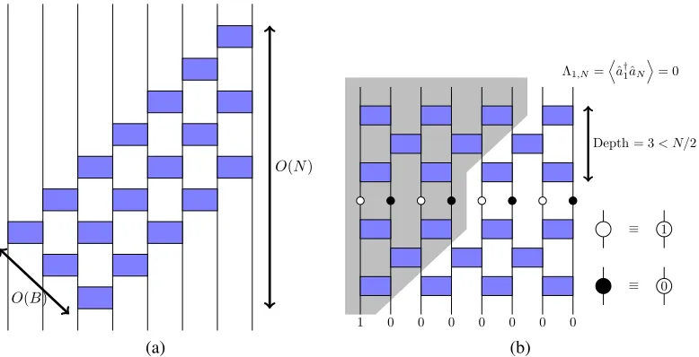
circuit has a depth ofO(N). However, a vertical cut through the circuit only passes throughO(B)gates. This construction and gate structure is in a certain sense optimal if we limit ourselves strictly to circuits with local gates. If we want to represent a correlation matrix in a compact way with nearest neighbor gates, we would like to be able to represent arbitrary correlations in the system (correlations at all lengths), and in particular, correlations between the first and last site. In Fig.25(b), we show a circuit which cannot connect the first and last sites because its depth is less than

(29)

O(N)

O(B)

(a)

Λ1,N= D

ˆ a†₁ˆaN

E

= 0

1 0 0 0 0 0 0 0

≡ 1

≡ 0

Depth = 3< N/2

[image:29.612.113.502.70.269.2]

(b)

Figure 25: Fig.25(a) shows the overall gate structure obtained by the diagonalization procedure. These gates form the total N × N unitary V which approximately diagonalizes our correlation matrixΛ. By conjugating a diagonal matrix with the appropriate occupations of 0 or 1 found in the diagonalization procedure by this set of gates, we get an approximation for the correlation matrix. Fig.25(b) shows an example of the correlations allowed by representing the correlation matrixΛwith a diagonal matrix conjugated by a finite depth circuit of depth< N/2. The grey area (the “light cone") represents sites where there can be nonzero correlations with the first site. The circles in the middle represent a diagonal matrix with 1’s and 0’s on the diagonal, which is conjugated by a unitary change of basis approximated here by a finite depth circuit. For the circuit depth shown, there can’t be correlations with the last two sites. A circuit of depth≥ N/2 is required to allow for the possibility of nontrivial correlations across the entire system.

to perform it again for another correlation matrix which is only locally different from the first one. If we choose the gauge center where the correlation matrix has changed, we only need to change a local set of gates.

A generic local circuit of depthO(N)contains O(N2)gates, and can represent an arbitrary N × N single-particle unitary change of basis. The low entanglement of physical ground states allows us to represent an N × N matrix with O(BN) one-parameter gates, withB N. For a gapless system, we know from conformal field theory that the entanglement of a subblockBofBsites varies asSB ∼log(B). This

means that we should be able to capture the entanglement of a critical system of N

(30)

2.3.2 Compressing a Correlation Matrix as a GMERA

A MERA tensor network[16] can represent a 1D critical system using a constant bond dimension, unlike an MPS. In our MPS construction, this is reflected in that

B∼log(N). However, we can adjust the diagonalization procedure slightly to obtain a MERA-like gate structure with a B which does not grow with N. The MERA for fermionic Gaussian states was first studied in [10], but was only used to study infinite translationally invariant systems and required a subtle optimization scheme. Here we will show a simpler construction only requiring the tools we have explained so far.

We begin the procedure in the same way as we did for the GMPS, by diagonalizing the block corresponding to sites 1, . . . ,Bof the correlation matrix. Just as before, for a large enough block size we find an occupied or unoccupied mode and rotate into the basis containing that mode withB−1 local 2×2 gates. Next, instead of diagonalizing the block starting at site 2, we instead diagonalize the block corresponding to sites 3, . . . ,B+2, again finding an occupied or unoccupied mode and rotating into that basis. The state at site 2 is “left behind"—it is not a low entangled state, so we cannot ignore it, but we leave it for a later stage of the algorithm. We continue in this manner, diagonalizing blocks starting at odd sites of size Bto obtain∼ BN/2 nearest neighbor gates. Approximately half of the modes are fully occupied or unoccupied and are projected out (meaning the associated rows and columns in the correlation matrix are ignored in later stages). The other half were left behind, and continue as the sites of the next layer of the gate structure. By only trying to get

N/2 unentangled modes in the first layer, the size of Bdoes not need to grow with

N, as we show below.

(31)

. . .

..

[image:31.612.142.458.87.318.2]

.

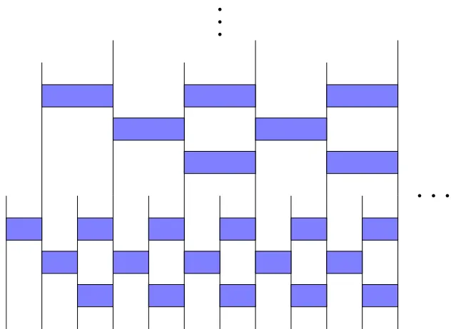
Figure 26: An example of an alternative diagonalization scheme resulting in a MERA-like gate structure. Here we show a section of the first two renormalization steps, with 12 sites shown in the first layer and 6 renormalized sites shown in the second. A block size of B = 4 is used. For this block size there are two layers of disentanglers and one layer of isometries per level of the MERA. Open legs at the top of each layer correspond to diagonal modes of the correlation matrix (with eigenvalues 0 or 1) and are ignored at the next layer.

in product states, meaning that swapping does not require significant time.

(32)

GMPS construction to project out all of the leftover sites at the end.

How does the block sizeBof the GMERA compare to that in our GMPS construc-tion? We show numerically in Section2.4.2that for a simple gapless Hamiltonian the GMERA does indeed produce accurate results with a block size B = O(1), independent of the system size, making it much more efficient in the largeN limit.

2.3.3 Discrete Wavelet Transforms and Fermionic Gaussian MERA

We would like to point out the similarity between the MERA gate structure and orthogonal wavelet transforms (WT), such as the WTs that produce the well-known Daubechies wavelets [17, 18]. Of course, the development of wavelets has not been in a many particle context, and, for now, we restrict ourselves to the matrix interpretation of the diagrams. For compact wavelets, an orthogonal wavelet trans-form is a local unitary transtrans-formation. It is not usually represented in terms of two-site gates, but this representation turns out be be particularly convenient. To be specific, we start with the simplest nontrivial WT, the D4 Daubechies WT. This WT is defined by four coefficients {aj} for j = 1, . . . ,4 which characterize how

the D4 scaling function is related to itself at different scales through the equation

s(x)=Í

jaj

√

2s(2x− j). The matrix form of the WT is given by

© «

a1 a2 a3 a4 0 0 0 a4 −a3 a2 −a1 0 0 0

0 0 a1 a2 a3 a4 0

0 0 a4 −a3 a2 −a1 0

. . . ª ® ® ® ® ® ® ® ® ¬ . (2.8)

The {aj} are carefully chosen to ensure orthogonality between scaling functions

centered at different sites, and to make the scaling functions have desirable com-pleteness properties. For example, linear combinations of the D4 scaling functions centered at different sites, {s(x − k)} for integer k, fit any linear function, so the resulting coefficients are a®T = (1+

√

3,3+

√

3,3−√3,1−√3)/(4

√

2). The or-thogonality requirement results in nonlinear equations to solve for the {aj} which

becomes complicated for higher order. The second row of the matrix gives the coefficients that produces wavelets, designed to represent high momentum degrees of freedom. In terms of our MERA procedure, the wavelets are left behind, while the scaling functions propagate to the next level.

(33)

s1 w1

θ1 θ1 θ1 θ1 θ1

θ2 θ2 θ2 θ2 θ2 θ2

s2 w2

θ1 θ1

θ2 θ2 θ2

. . .

[image:33.612.133.482.85.274.2]

..

.

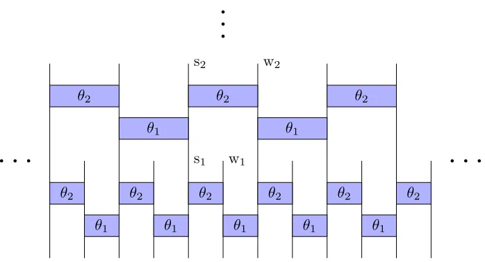
Figure 27: Here we show an example of a discrete wavelet transform written in the gate notation introduced in this paper. We show the D4 wavelet, which corresponds to a fermionic Gaussian MERA with one layer of disentanglers and one layer of isometries per layer. w1 and s1 (w2 and s2) label wavelet and scaling

functions for the first (second) layer. Taking θ1 = π/6 and θ2 = 5π/12, we

reproduce the conventional scaling coefficients for the D4 WT,a®T = (a1,a2,a3,a4)= (1+√3,3+√3,3−√3,1−√3)/(4

√

2).

gates have the same angle. The D4 WT is specified by only two angles, θ1 for the

bottom layer andθ2for the next. Higher order WTs of this type (e.g. D6, D8, etc.)

correspond to larger B. (For example, the D6 WT looks like Fig. 6). Given the angles, one gets the{aj} by setting all the top values of the circuit to zero except a

1 on one site and applying the 2×2 rotations in the layers below. The support of the scaling functions is made obvious using the gate structure, as there will be 2L

nonzero values at the bottom of the circuit forLlayers of gates. For the D4 WT, one finds thatθ1= π/6 and θ2 =5π/12 reproduces the D4{aj}, up to a trivial reversal

of the coefficients. (A single layer with θ1 = π/4 gives the trivial Haar wavelets,

which have been used previously as a basis for transforming fermionic Gaussian states by Qi [19].) The scaling functions at the larger scales are found by performing the same transformation of L layers of gates on the scaling functions found at the previous scale.

In Fig. 28 we show how scaling coefficients {aj} come from the gate structure,

(34)

0

1

0







c

₁

₋

s

₁

s

1

c

1

c

1

−

s

1

s

₁

c

₁













1 c

2

−

s

2

s

2

c

2

1 











0

1

0

0 





=







a

₄

i

= sin(

θ

i

)

(b) Gate structure in (a) written in terms of matrices and vectors.

0

1

0 θ

₁

θ

(c) Wavelet coefficients from gate structure.

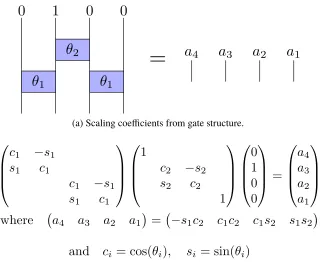
Figure 28: Here we show explicitly how to obtain the scaling and wavelet coefficients of the D4 WT from the circuit construction. Taking θ1 = π/6 and θ2 = 5π/12,

in (a) and (b) we reproduce the conventional scaling coefficients for the D4 WT,

®

aT = (a1,a2,a3,a4)=(1+ √

3,3+

√

3,3− √

3,1− √

3)/(4

√

(35)

are obtained by shifting the location of the 1 at the top of the circuit, but we can show in general that this gives the same result. This is done by noting that the shift of the 1 to get the wavelet coefficients looks like a swap at the top of the circuit. We can “pull through" this swap by conjugating each layer of the WT with a transformation that reverses the order of the sites. This conjugation also negates the angles in the circuit. It leaves a site reversal at the bottom of the circuit, reversing the order of the coefficients. The angle negation negates the sine terms, leading to the same coefficients except with every other one negated, since every other site will have an even or odd number of sin(θ_i)multiplied together.

Given an arbitrary set of {aj}, we can use the same procedure that brought ®v to

the first site in our GMPS procedure to find all the angles defining the WT, i.e

®

v = a®. Thus, any compact orthogonal WT of this general type can be represented by a simple gate structure. Because wavelets are much easier to understand than generic many particle wavefunctions, the connection between MERA and wavelets may help provide intuition that helps one understand MERA.

2.3.4 Forming the Many-Body MPS from the GMPS (or GMERA)

For a number conserving real Hamiltonian H, the many particle unitary gate ˆVi

corresponding to the single particle rotationVi, in the basis

{|Ωi,aˆ†_i |Ωi,aˆ†_i₊₁|Ωi,aˆ†_iaˆ_i†₊₁|Ωi}, (2.9)

is

[Vˆi]= [Vˆ(θi)]=

©

«

1 0 0 0

0 cosθi sinθi 0

0 −sinθi cosθi 0

0 0 0 1

ª ® ® ® ® ®

¬

. (2.10)

This reinterpretation of the gates is the only change needed to make our matrix gate structures act on the many particle Hilbert space.

Say we have compressed the correlation matrix of a pure fermionic Gaussian state as a GMPS. To create the MPS representation of this state, we begin with a product state, with each site being occupied or unoccupied, with the occupations given by

nk obtained in our diagonalization procedure (set to 1 or 0 fornk ≈ 1 or 0). We

then apply, one by one, all of the nearest neighbor gates{Vˆi} (the many-body gates

corresponding to the gates{Vi}obtained with Eq.2.10) in the opposite order in which

(36)

ˆ

VB1

ˆ

V_B2

ˆ

VB3

ˆ

VB4

ˆ

VB5

ˆ

V_B6

ˆ

VB7

=

[image:36.612.120.498.72.241.2]

=

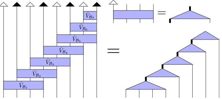
Figure 29: Tensor diagram showing the structure of gates{VˆBi}fori =1, . . . ,N−1 obtained in our procedure and how they contract to form an MPS. The white (black) triangles represent projectors onto the occupied (unoccupied) state. The ordering of the occupied and unoccupied states is determined by the ordering of the occupations found in the diagonalization procedure, one particular example at half filling is shown here. Here we show a system with N = 8 sites and a block size B= 4. The diagram on the right shows that once the sites are rotated into a basis where one of the modes is occupied or unoccupied (generally with some alternating pattern), the fully occupied or unoccupied modes can be projected out. The transformations

{VˆBi}, including the projections, can be directly interpreted as the tensors composing the MPS representation of our many-body state if we do an exact contraction, or we can apply them as a set of gates as explained in the text.

of gates is similar to the time-evolving block decimation (TEBD) algorithm[20] or the time dependent DMRG algorithm[21], but the pattern of gates and ordering is different. We apply the two body gates by moving the center of the MPS to the location of the gate, contract the gate with the two relevant tensors in the MPS, and then form the new MPS by performing a singular value decomposition (SVD), with possible truncation of states by throwing out states with small singular values.

We can also form the MPS from our GMERA construction in a similar manner. However, instead of starting with a full product state, we start with the gates at the top of the MERA and work our way down, including only the sites that have been touched by a gate at that level or above. When a site is added, it starts as a completely occupied or unoccupied state, and is immediately mixed with another site by a gate. The number of sites involved roughly doubles with each layer, and afterO(log₂(N))

(37)

Returning to the MPS construction, the tensors of the MPS could also be constructed directly by contractions of the gates as shown in Fig.29. In this diagram the small black and white triangles signify projectors onto the appropriate occupations found, while the thick lines signify combined internal indices which form the internal bonds of the MPS. From this perspective it is easy to see that picking a block sizeB

for diagonalizing the correlation matrix would correspond to an MPS with a bond dimension of χ = 2B−1. We find it simpler and more efficient to apply the gates layer by layer instead of this method. Layer by layer, it is natural to truncate the MPS with SVDs during the construction, and this can lead to an MPS with a smaller bond dimension than 2B−1for the required accuracy. The SVD truncation takes one out of the manifold of Gaussian states, where the greater freedom for a fixed bond dimension allows one to find a state which is closer to the desired Gaussian state than one could within the Gaussian manifold. However, one should pick a block size so that 2B−1is as close to the target bond dimension as possible.

We can adapt our circuits to complex quadratic Hamiltonians, where the gates are of the same form but the 2×2 submatrix rotating the singly occupied subspace is a general matrix in SU(2) parameterized by two angles. Even more generally, we can extend this procedure to quadratic Hamiltonians with pairing terms to compress BCS states, where the gates required are not just number conserving but general parity conserving gates (so they involve mixing of unoccupied and doubly occupied subspaces of the 2 sites of interest). This matrix would in general be parameterized by 5 angles (one matrix in SU(2) rotating the singly occupied subspace, one matrix in SU(2) rotating the empty and doubly occupied subspaces, and a relative phase). This form of gates has been studied previously in the context of classically simulating quantum circuits using the matchgate formalism; see for example[22,23].

2.4 Numerical Results

Here we show numerical results for the algorithms we presented. In order to study systems that are both gapless and gapped, we study a simple model, the Su-Schrieffer-Heeger model [24]. This is a model of 1D spinless fermions hopping on a lattice with staggered hopping amplitudes,t1andt2. The Hamiltonian is

ˆ

HSSH =

N−1 2

Õ

i=1

(t1aˆ₂†_i−1aˆ2i+t2aˆ

†

2iaˆ2i+1+h.c.). (2.11)

We will take t1 = −t 1+ δ₂

and t2 = −t 1− ₂δ

(38)

2

4

6

8

10

0

1

2

3

4 Blo

ck

size

B

[image:38.612.128.472.73.323.2]

Energy gap

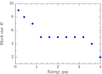
Figure 210: Block size required to obtain a relative error in the total energy of less than 10−6as a function of the calculated energy gap (in units oft) forN = 128 sites.

thermodynamic limit (N → ∞). With open boundary conditions, it can contain exponentially decaying zero energy modes localized on the ends of the chain.

2.4.1 Results for Compressing a Correlation Matrix as a GMPS

We start with a simple test of obtaining the GMPS compression of the ground state correlation matrix of the SSH model for N = 128 lattice sites for various energy gaps at half filling (NF = N/2). We analyze the range of δ from 0 to 2.

The ground state for δ = 0 is (approximately) gapless while for δ = 2 it is fully gapped (the chain uncouples). Fig. 210 shows the block size required to obtain a GMPS with a relative error in the total energy of less than 10−6as a function of the calculated energy gap. The exact ground state energy and energy gap are calculated by diagonalizing the hopping HamiltonianHSSH. This corresponds to the accuracy

of the MPS representation of the ground state if the GMPS written with many-body gates is contracted with no further truncation of the MPS, so a GMPS block size B

(39)

1e-07

1e-06

1e-05

0.0001

0.001

0.01

0.1

2

4

6

8 Relativ

e

error

in

energy

[image:39.612.129.474.104.351.2]

Block size

B

Figure 211: Relative error in the total energy as a function of the block size B for

N =128 sites andδ =0.

-0.5 0 0.5

20 40 60 80 100

Amplitude

of

mo

de

Site

n1≈1 n42≈0 n85≈1

(a)δ=0.4 (energy gap≈0.806135t)

-0.5 0 0.5

20 40 60 80 100

Amplitude

of

mo

de

Site

n1≈1 n41≈1 n85≈1

(b)δ=0 (energy gap≈0.146088t)

[image:39.612.113.504.469.618.2]

(40)

0 0.5e-07

25 50 75 100 125

Deviation

in

eigen

value

nk

Modek

B= 7

(a)δ=0.4 (energy gap≈0.806135t)

0 0.5e-07 1e-07 1.5e-07 2e-07

25 50 75 100 125

Deviation

in

eigen

value

nk

Modek

B= 9

[image:40.612.112.504.84.231.2]

(b)δ=0 (energy gap≈0.146088t)

Figure 213: Examples of deviations in occupations at the end of the diagonalization procedure forN = 128 sites. Fig.213(a) shows errors in the occupations forδ =0.4 (energy gap≈0.806135t). Fig.213(b) shows errors in the occupations forδ = 0.0 (energy gap≈0.146088t).

Fig.212shows examples of the modes obtained with the procedure, both filled and unfilled, for a small gap and a larger gap. The modes are seen to be localized for the case of the larger gap, and extend throughout the system for the smaller gap. The unfilled modes follow the same decay as the filled modes but oscillate more, since they are above the Fermi sea and are therefore higher in energy. Fig.213shows for the same two gaps the deviation in the eigenvaluesnk from 0 or 1 obtained during

the diagonalization procedure. For the case of the larger gap, this error saturates to its maximum quickly for modes near the middle of the system, while for the smaller gap, the error increases more slowly due to the longer range correlations.

In Fig. 214 we analyze the block size scaling with system size N for the gapless case (δ = 0). As we expect from arguments about entanglement made at the end of Section 2.3.1, the scaling is found to be B ∼ log(N). This is the expected scaling for a critical 1D system. We can see that with this procedure we can analyze very large systems, up to N = 216 = 65536 sites, even for gapless free fermions. To avoid storing correlation matrices this large, we begin with a very accurate compressed correlation matrix as a GMPS using the GDMRG algorithm presented in Appendix 2.B. With GDMRG, we begin with a state with a relative error in the energy of < 10−10. For N = 65536 this requires a block size of

(41)

6

8

10

12

14

16

size

B

[image:41.612.132.472.74.324.2]

Number of sites

N

Figure 214: Block size Bneeded for a relative error in the energy of < 10−6 as a function of number of sites N for spinless, gapless fermions with open boundary conditions at half filling. As expected from arguments about the entanglement of a critical system, we find B ∼ log(N), tested up to N = 216 = 65536 sites (note the log scale on the x axis). To study systems of this size and avoid the O(N3)

diagonalization of the hopping Hamiltonian, we obtain the correlation matrix using the GDMRG algorithm as explained in Appendix2.B.

from GDMRG, because GDMRG optimizes the energy which only depends on very local correlations.

2.4.2 GMERA Results

Here we present results for compressing a correlation matrix as a GMERA using the procedure presented in Section2.3.2. We show the relative error in the energy for increasing number of sites for B = 10 in Fig.215. We see that for this block size, the error stays below 10−6 for systems up to N = 214 = 16384 and in fact appears to saturate at high number of sites (the change in the relative error in the energy approaches 0 for larger system sizes). This is in stark contrast to the GMPS, where a block sizeB ∼log(N)was required to obtain a fixed accuracy, as shown in Fig.214. Instead, the GMERA obtains the same accuracy with constant block size

(42)

0 1e-07

2e-07

3e-07

4e-07

5e-07

Relativ

e

error

in

energy

Number of sites

N

[image:42.612.131.473.73.322.2]

B = 10

Figure 215: Relative error in the energy for the proposed GMERA construction for increasing number of sites for a block size B = 10. The system analyzed is the ground state of free fermions hopping on a lattice with open boundary conditions. All errors are below 10−6. As expected for a MERA, the error is seen to saturate for large N, indicating a fixed block size is sufficient to obtain an accuracy < 10−6up to very large system sizes.

made possible partially because the GMERA structure involves nonlocal gates.

2.4.3 GMPS to Many-Body MPS Results

Plots of the time it takes to form the MPS of the ground state of a gapless free fermion system for up to N = 1024 sites using the method presented in Section 2.3.4 are shown in Fig.216. As expected, the time it takes for a gapless system is polynomial in the system sizeN, while it is approximately linear in Nfor a gapped system. The SSH model is used withδ = 0.1 or an energy gap ∆≈ 0.2t. The time to form the gapless ground state is only a modest polynomial inN,∼ N2.03, while as we expect from arguments about entanglement the time to form the gapped ground state is very nearly linear in N, ∼ N1.02, because the block size and bond dimension required to obtain the specified accuracy are constant for all N shown (B = 8 and χ = 55). With this method, a gapless ground state of N = 1025 sites with a relative error in the energy of< 10−6can be formed on a laptop in only∼ 90 seconds.

(43)

0

20

40

60

80

100

225

425

625

825 1025

Time

to

form

MPS

(s)

Number of sites

N

Gapless,

_∼

N

2.03

Gapped,

_∼

N

1.02

B

= 11,

χ

= 364

[image:43.612.113.488.78.349.2]

B

= 8,

χ

= 55

Figure 216: A plot of the time to form the MPS approximation of gapped and gapless free fermion ground states at half filling as a function of sitesN using gates from a GMPS. The bond dimensions are chosen large enough such that the relative errors in the energy of the MPS are below 10−6. The block size of the GMPS used to form the MPS are the minimum required to obtain a GMPS with a relative error in the energy of 10−6. A cutoff in the singular values of the SVD of 10−11was used when applying the gates to form the MPS using the method described in Section2.3.4. For the gapped case, the SSH model withδ = 0.1 is used, corresponding to an energy gap of∆≈0.2t (exact asN → ∞).

(44)

are used, as we do here), so through the SVD we are able to compress the state quite efficiently beyond what we initially might expect.

2.5 Conclusion

We have presented an efficient, numerically stable, and controllably accurate way to compress a correlation matrix into a set of 2× 2 unitary gates. From these gates, we have also presented a method for easily and efficiently forming the MPS approximation of a fermionic Gaussian state. We explained the procedure in detail for the ground state of a generic number conserving Hamiltonian. We then presented results for the SSH model, a 1D chain of fermions with staggered hopping. We showed examples of the accuracy and block sizes needed for different gaps of the model. We hope this method can be used as a simple, efficient and reliable procedure for directly preparing many states of interest, either by creating starting states to aid DMRG calculations or preparing a particular ansatz as an MPS. We also presented one example of how the procedure can be modified to obtain different gate structures, in this case one that is related to the MERA. However, there are other possibilities to be explored, such as gate structures more directly suited for systems with 2 spatial dimensions, periodic boundary conditions, as well as how the method might be applied to study thermal fermionic Gaussian states. In addition, we presented how discrete wavelet transforms can be described very simply with the gate structure notation we introduced in this paper.

(45)

APPENDIX

2.A Calculation of the Entanglement Entropy of a Fermionic Gaussian State

In this section we give a simple, self-contained derivation for Eq.2.6, the entangle-ment entropy for a block of a free fermion system. This expression has been shown elsewhere[12–15], though we show a simple, self-contained derivation here.

Assume the block of interestBis the firstBsites. Gaussian states have expectation values that obey Wick’s theorem. This means that the expectation value of any operator contained within the block is specified if we know subblock B of the correlation matrix, ΛB. This implies that the many-body density matrix of the block ˆρB is also uniquely specified by ΛB. The entanglement entropy on block

B, defined as SB[ρˆB] = −Tr[ρˆBlog(ρˆB)], does not change under general unitary transformations within the block. Thus, we can perform the single particle unitary transformation of basis that makesΛB diagonal, with diagonal entriesnb=

D ˆ

a†_baˆb

E

for b∈ 1, . . . ,B. Thenbuniquely specify the reduced density matrix of the block,

so the entanglement is a universal function of{nb}:

SB = SB(n1, . . . ,nB). (2.12)

In fact, the details of the system outside the block are irrelevant. For example, different systems with different numbers of sites outside the block can have the same

SB as long as their {nb} are identical and the system is a Gaussian state. Thus to

evaluate the function SB, we can choose a simple system in which to evaluate it

rather than using the actual system of interest.

Let’s first consider a block with only one site (B = 1). We would like to know the universal functionS1(n1). We choose a two site system containing a single particle, with normalized wavefunction

|ψi= (√n1aˆ†₁+

p

1−n1aˆ†₂) |Ωi. (2.13)

The correlation matrix is

n1 pn1(1−n1)

p

n1(1−n1) 1−n1

!

, (2.14)

which has the required block correlation matrixΛ1= (n1). The Schmidt

decompo-sition of|ψiis

|ψi= p1−n1(|0i)(aˆ†₂|0i)+√n1(aˆ†₁|0i)(|0i)

= p

1−n1|0i |1i+ √

n1|1i |0i,

Development of Tensor Network Algorithms for Studying Classical and Quantum Many Body Systems

Classical and Quantum Many-Body Systems

Matthew Theodore Fishman

ACKNOWLEDGEMENTS

ABSTRACT

PUBLISHED CONTENT AND CONTRIBUTIONS

CONTENTS

LIST OF FIGURES

INTRODUCTION

FREE FERMION DENSITY MATRIX RENORMALIZATION

GROUP

-0.5

0

0.5

5

10

Amplitude

of

mo

de

Site

≡

















1

1

1

1

















V

(

θ

)

V

(

θ

) =

cos

θ

−

sin

θ

sin

θ

cos

θ

V

(

θ

)

Λ

~v

≈

n

~v

,

n

≈

1

. . .

..

.

. . .

. . .

..

.

0

_≈

₋