A comparative study on optimal structural dynamics using wavelet functions

(1)

Research Article

A Comparative Study on Optimal Structural

Dynamics Using Wavelet Functions

Seyed Hossein Mahdavi and Hashim Abdul Razak

StruHMRS Group, Department of Civil Engineering, University of Malaya, 50603 Kuala Lumpur, Malaysia

Correspondence should be addressed to Hashim Abdul Razak; [email protected]

Received 2 April 2014; Accepted 8 October 2014

Academic Editor: Shuenn-Yih Chang

Copyright © 2015 S. H. Mahdavi and H. Abdul Razak. This is an open access article distributed under the Creative Commons Attribution License, which permits unrestricted use, distribution, and reproduction in any medium, provided the original work is properly cited.

Wavelet solution techniques have become the focus of interest among researchers in different disciplines of science and technology. In this paper, implementation of two different wavelet basis functions has been comparatively considered for dynamic analysis of structures. For this aim, computational technique is developed by using free scale of simple Haar wavelet, initially. Later, complex and continuous Chebyshev wavelet basis functions are presented to improve the time history analysis of structures. Free-scaled Chebyshev coefficient matrix and operation of integration are derived to directly approximate displacements of the corresponding system. In addition, stability of responses has been investigated for the proposed algorithm of discrete Haar wavelet compared against continuous Chebyshev wavelet. To demonstrate the validity of the wavelet-based algorithms, aforesaid schemes have been extended to the linear and nonlinear structural dynamics. The effectiveness of free-scaled Chebyshev wavelet has been compared with simple Haar wavelet and two common integration methods. It is deduced that either indirect method proposed for discrete Haar wavelet or direct approach for continuous Chebyshev wavelet is unconditionally stable. Finally, it is concluded that numerical solution is highly benefited by the least computation time involved and high accuracy of response, particularly using low scale of complex Chebyshev wavelet.

1. Introduction

Generally, results integrated from dynamic analysis of struc-tures are the main reliable criteria for design of solids and structures. The technique for a solution of general dynamic equilibrium can become very expensive if a com-plex loading (e.g., an unknown earthquake excitation) is being applied on large-scaled structures [1, 2]. In general, procedure of dynamic analysis is categorized into the two solution methods: first, mode superposition method. Second, direct and indirect integration methods, for example, central differences, family of Newmark-𝛽, Houbolt, and Wilson-𝜃fall under direct integration schemes and Fourier transformation and wavelet analysis have been introduced as indirect integra-tion approaches. In addiintegra-tion, the choice as to which method to use for an effective solution is governed by the dynamical problem considered [3,4]. Theoretically, aforesaid numerical integration methods lie in case of either conditionally stable or unconditionally stable procedures. An integration method

is unconditionally stable if the solution for any initial condi-tions does not grow without a band for any time step while will be conditionally stable if it does grow. In other words, stability of results is achieved at any time interval and there is no restriction on usingΔ𝑡smaller than a particular value. As a result, optimal solution for dynamic analysis is accomplished using long intervals [5–7].

Nowadays, orthogonal polynomials are being widely implemented as a practical analysis of time dealing problems in engineering, particularly in the form of wavelet analysis. Obvious effectiveness from property of orthogonality is that the repeated components with similar characteristics are neglected in the analytical process [8, 9]. Consequently, computational calculations are being considerably decreased and computation time involved is being therefore reduced, hence, accuracy of responses will be more desirable [10,11]. Practically, considerable attention has been given for the use of wavelet method for the solution of time dependent prob-lems such as dynamic analysis or identification of systematic

(2)

problems [12]. Several attractive mathematical characteris-tics of wavelets such as efficient multiscale decompositions, localization properties in physical and wave-number spaces, and the existence of recursive and fast wavelet transforms have obtained practice of this efficient tool for the numerical solution of partial differential equations (PDEs) and ordinary differential equations (ODEs) [13–15].

Significantly, accuracy of responses is directly related to the basis function of mother wavelet, depending on the kind of objectives. Fundamentally, in the structural dynamics, compatibility of a wavelet basis function is premised upon on not only the degrees of freedom but also the similarity of basic functions to the lateral loading, emphasizing on frequency contents. Considerably, less computational cost of calculations in advanced time history analysis through the compatible wavelet functions makes distinction of this approach over other numerical methods. For instance, for the purpose of time history analysis, a simple basis function of Haar wavelet was indirectly applied on its own free-scaled functions [16]. It is inferred that because of the inherent simple shape function of Haar wavelet accuracy of responses was undesirable even employing large-scaled functions. Furthermore, to improve inadequacy of Haar wavelet known as the simplest and two-dimensional (2D) wavelet basis function, it is indispensable to employ three-dimensional (3D) and adaptive wavelet basis functions [17, 18]. Moreover, there is no consideration reported on the stability of responses calculated using Haar wavelet functions compared with other basis functions.

Mathematically, adaptive wavelets are those that grow in three dimensions, which in the current definition dimensions are time, scale, and frequency, respectively. For instance, Chebyshev, Legender, and Symlet are some basis functions with compatible characteristics [19]. Basically, Chebyshev polynomials are presented as continuous basis function of wavelet [20, 21]. The most popular characteristic of this wavelet is various weight functions of Chebyshev polynomi-als that directly influence stability and accuracy of responses [22–24]. However, it is reported that stability of results computed by Chebyshev wavelet are independent from initial accelerations. Furthermore, compatibility is being satisfied through the capturing of broad frequency of complex excita-tions by oscillated shape funcexcita-tions of free-scaled Chebyshev wavelet [25].

Subsequently, the main contributions of this study (which received little attention in the literature) are composed of the following: (i) a numerical assessment of structural dynamic problems using free-scaled simple and complex wavelet functions, with the emphasis on the large scales of wavelets, (ii) numerical stability analysis of an indirect algorithm using family of discrete Haar wavelets, established as 2D wavelet functions, (iii) stability analysis of continuous Chebyshev wavelet functions with respect to the third-ordered derivation of time, (iv) a comparative evaluation of computational efficiency of simple and complex wavelets for smooth and wide-band frequency contents of loading, and (v) capability evaluation of Haar and Chebyshev wavelets in linear and nonlinear structural dynamic problems. Accord-ingly, to achieve the proposed objectives of this paper,

the second-ordered differential equation of motion is indi-rectly solved by free scale of Haar wavelet and later, free-scaled Chebyshev wavelet functions are directly implemented to compute responses. For this aim, a brief background of wavelet is discussed inSection 2of this study. In addition, coefficient matrices of wavelet and operation matrices of inte-gration corresponding to complex scales of efficient Cheby-shev wavelet are formulated and presented in this section. In Section 3, the computational procedure is developed for an optimal dynamic analysis.Section 4is allocated to numerical stability analysis of responses, corresponding to the indirect method proposed for Haar and direct scheme proposed for Chebyshev wavelet functions. Accordingly, stability of responses has been comparatively presented. Section 5 is devoted to investigation of the validity and effectiveness of results. For this purpose, various scales of Chebyshev and Haar wavelet functions are considered for dynamic analysis. Finally, efficiency and accuracy of results have been compared in this section.

2. Fundamental of Wavelet

2.1. Haar Wavelet. The simple family of Haar wavelet was presented by Alfred Haar in 1910 for𝑡 ∈ [0, 1] as follows [16,18]:

𝐻_𝑚−1(𝑡) =

{ { { { { { { { { { { { {

1, 𝑡 ∈ [₂𝑘_𝑗 , 𝑘 + 0.5₂_𝑗 ] ,

−1, 𝑡 ∈ [𝑘 + 0.5₂_𝑗 , 𝑘 + 1₂_𝑗 ] ,

0, otherwise,

(1)

where

𝑚 = 2𝑗+ 𝑏 + 1, 𝑗 ≥ 0, 0 ≤ 𝑏 ≤ 2𝑗− 1, (2)

where𝑀 = 2𝑗 (𝑗 = 0, 1, . . . , 𝑗)denotes the order of wavelet;

𝑏 = 0, 1, . . . , 𝑀 − 1is the value of transition. In(1),𝑚 = 1

and 𝑚 = 2indicate scale function and mother wavelet of

Haar, respectively. In this study,2𝑀indicates the number of segmentations in each global time interval regarding the scale of proposed wavelet which refers to segmentation method (SM). For example, in the case of Haar wavelet2𝑀 = 2𝑗+1 denotes the2𝑗th scale of Haar wavelet [18].

Basically, signal𝑓(𝑡)can be expanded in Haar series as [16]:

𝑓 (𝑡) ≅2𝑀∑

𝑖=0

𝑐_𝑖ℎ_𝑖(𝑡) . (3)

Accordingly, Haar coefficients 𝑐_𝑖 (𝑖 = 0, 1, 2, . . .) are defined by

𝑐𝑖= 2𝑗∫

1

0 𝑓 (𝑡) ℎ𝑖(𝑡) 𝑑𝑡. (4)

Hence,𝐻_2𝑀is a square matrix(2𝑀 × 2𝑀), including the first2𝑀scale of Haar wavelet; Haar coefficients are directly given as

𝑐_𝑖= 𝑓 (𝑡) 𝐻−1

(3)

Equivalently, signal𝑓(𝑡)may be rewritten as

𝑓 (𝑡) ≅ 𝑐𝑇

2𝑀𝐻2𝑀(𝑡) . (6)

Subsequently, integration of 𝐻_2𝑀 is obtained by Haar series with new square coefficient matrix of integration𝑃_2𝑀 as [16,18]

∫1

0 𝐻2𝑀(𝑡) 𝑑𝑡 ≈ 𝑃𝐻2𝑀(𝑡) . (7)

Pointed out that local times are calculated relatively to the scale of wavelet as

𝜏𝑙= 𝑙− 0.5_2𝑀 , 𝑙 = 1, 2, . . . , 2𝑀. (8)

Finally, the local time divisions (𝜏_𝑙) are adapted to the global domain. Assumption of𝑑_𝑡as global time interval we have [16,18]

𝑡𝑙𝑡 = 𝑑𝑡(𝜏𝑙) + 𝑡𝑡󳨐⇒ 𝜏𝑙= 𝑡𝑡− 𝑡_𝑑 𝑙𝑡

𝑡 , 𝑙 = 1, 2, . . . , 2𝑀. (9)

2.2. Chebyshev Wavelet. In mathematics, families of contin-uous wavelet transforms (CWT) are considered as follows [22,24]:

CWT(Scale,Position)

= ∫ 𝑓 (𝑡) Ψ (Scale,Position) 𝑑𝑡,

(10)

where CWT denotes corresponding wavelet transform. As long as wavelet functionΨ(𝑡)is supposed as mother wavelet, the continuous wavelet transform of a signal𝑓(𝑡)is obtained as

CWTΨ_𝑆 (𝑎, 𝑏) = 1

√|𝑎|∫ 𝑓 (𝑡) Ψ

∗

𝑎,𝑏(𝑡) 𝑑𝑡, (11)

where𝑏, 𝑎indicate the transition and the scale of wavelet and

∗indicates the complex conjugate form ofΨ(𝑡), respectively. In general, the Chebyshev polynomials, named after Pafnuty Chebyshev, are a sequence of orthogonal polyno-mials defined as two kinds. The general expression for Chebyshev polynomials of the first kind (𝑇_𝑛) is defined as follows [20,21]:

𝑇𝑛(𝑥)

= (𝑛₂)𝑛/2∑

𝑘=0((−1)

𝑘𝑛 − 𝑘 − 1!

𝑛 − 2𝑘!𝑘! × (2𝑥)𝑛−2𝑘) ,

𝑛 = 1, 2, 3, . . ..

(12)

In addition, the variable weight functions of𝑇_𝑛is defined as𝜔_(𝑥)[25]

𝜔(𝑥)=

{ { {

1

√1 − 𝑥2, |𝑥| < 1,

0, |𝑥| ≥ 1. (13)

Mathematically, the Chebyshev wavelet arguments are defined as

Ψ_𝑛,𝑚= Ψ (𝑘, 𝑛, 𝑚, 𝑡) ,

𝑛 = 1, 2, . . . , 2𝑘−1, 𝑚 = 0, 1, . . . , 𝑀 − 1, 𝑘 = 1, 2, 3, . . . ,

(14) where positive integer 𝑘denotes the value of transition, 𝑡 indicates the time,𝑚is degree of Chebyshev polynomials for the first kind, and𝑛denotes the considered scale of wavelet. Chebyshev wavelets are formulated with substituting the first kind 𝑇_𝑛 with relevant weight functions for each scale and transition in(11)as follows [22,25]:

𝜓_𝑚(𝑡)

={{_{_{

{

(2𝑘/2) × 𝑇_𝑚(2𝑘(𝑡) − 2𝑛 + 1) , 𝑛 − 1

2𝑘−1 < 𝑡 ≤

𝑛

2𝑘−1,

0 Otherwise,

(15) where𝑇_𝑚in(15)is obtained as

𝑇_𝑚(𝑡) =

{ { { { { { {

1

√𝜋, 𝑚 = 0,

𝑇_𝑚× √_𝜋2, 𝑚 > 0. (16)

Thus, weight functions corresponding to different scales are obtained as

𝜔_𝑛(𝑡) = 𝜔 (2𝑘⋅ 𝑡 − 2𝑛 + 1) . (17)

Regarding the idea of SM method 𝐷 is number of partitions in the global time,𝑀is the order of Chebyshev polynomials that is derived as

2𝑘−1𝑀 = 𝐷 󳨐⇒ 𝑀 = 𝐷

2𝑘−1. (18)

Numerically, the signal𝑓(𝑡)can be expanded with Cheby-shev wavelets as [19,22]

𝑓 (𝑡) ≈2

𝑘−1

∑

𝑛=1 𝑀−1

∑

𝑚=0

𝐶_𝑛,𝑚𝜓_𝑛,𝑚(𝑡) = 𝐶𝑇⋅ 𝜓 (𝑡) . (19)

Here,𝐶and𝜓(𝑡)are obtained as two vectors:

𝐶 = [𝑐₁, 𝑐₂, 𝑐₃, . . . , 𝑐₂𝑘−1]𝑇₂𝑘−1_𝑀×1, (20)

where

𝐶_𝑖= [𝑐_𝑖0, 𝑐_𝑖1, 𝑐_𝑖2, . . . , 𝑐_{𝑖,𝑀−1}]𝑇. (21)

Chebyshev coefficients matrix is defined as

(4)

where

𝜓_𝑖(𝑡) = [𝜓𝑖0(𝑡) , 𝜓𝑖1(𝑡) , 𝜓𝑖2(𝑡) , . . . , 𝜓𝑖,𝑀−1(𝑡)]𝑇, (23)

where𝑖 = 1, 2, 4, . . . , 2(𝑘−1).

Local time 𝑡_𝑙 for collocation points are considered as follows [25]:

𝑡𝑙= (₂_𝑘−11_𝑀) (𝑙− 0.5) , 𝑙 = 1, 2, 3, . . . , 2𝑘−1𝑀. (24)

Subsequently, a 𝐷 × 𝐷-dimensional square matrix of

𝜙_𝑛,𝑚(𝑡)is derived as

𝜙_𝑛,𝑚(𝑡) = [𝜓 (𝑡₁) 𝜓 (𝑡₂) ⋅ ⋅ ⋅ 𝜓 (𝑡_𝑖)]₂𝑘−1_𝑀×2𝑘−1_𝑀. (25)

For instance, assumption of 𝑀 = 4 and 𝑘 = 2; lies on the first four equations of Chebyshev wavelet cor-responding to eight collocation points (in referring to the SM method). Accordingly, coefficient matrix of free-scaled Chebyshev wavelet of𝜙_8,8(𝑡)corresponding to2𝑀local times is improved as follows:

𝜙_𝐷×𝐷

= [ [ [ [ [ [ [ [ [ [ [ [ [ [ [ [ [ [ [ [ [ [ [ [ [

𝜓₁₀ 𝜓₁₀ 0 ≤ 𝑡 < 0.5 𝜓₁₀ 𝜓₁₀ ... 𝜓₁₀ 𝜓₁₀ 0.5 ≤ 𝑡 < 1 𝜓₁₀ 𝜓₁₀

𝜓₁₁ 𝜓₁₁ . . . 𝜓₁₁ 𝜓₁₁ ... 𝑛 − 1

2𝑘−1∢𝑡local∢

𝑛

2𝑘−1

𝜓₁₂ ... ZERO

𝜓₁₃ 𝑛 = 1 d ... 𝑛 = 1

⋅ ⋅ ⋅ ⋅ ⋅ ⋅ ⋅ ⋅ ⋅ ⋅ ⋅ ⋅ ⋅ ⋅ ⋅ d ⋅ ⋅ ⋅ ⋅ ⋅ ⋅ ⋅ ⋅ ⋅ ⋅ ⋅ ⋅ ⋅ ⋅ ⋅

𝜓₂₀ 𝜓₂₀ ⋅ ⋅ ⋅ 𝜓₂₀ 𝜓₂₀ ... d ⋅ ⋅ ⋅

𝜓₂₁ 𝑛 − 1

2𝑘−1∢𝑡local∢

𝑛

2𝑘−1 ...

𝜓₂₂ ZERO ...

𝜓₂𝑘−1_×𝑀−1 𝑛 = 2 ... 𝑛 = 2 𝜓₂𝑘−1_×𝑀−1

] ] ] ] ] ] ] ] ] ] ] ] ] ] ] ] ] ] ] ] ] ] ] ] ]

, (26)

where

in 𝜓_𝑛,𝑚󳨀→ 𝑛 = 1, 2, . . . , 2𝑘−1,

𝐷 = 2𝑘−1× 1. (27)

Local times(𝑡_𝑙)for𝑀 = 4and𝑘 = 2are calculated on

2𝑀 = 8points as

𝑡_𝑙= [0.0625; 0.1875; 0.3125; 0.4375; 0.5625; 0.6875;

0.8125; 0.9375] . (28)

As can be seen from the matrix of (26), column of𝑖th refers to𝜓_𝑖and integration of𝜓(𝑡)in the local time is obtained as

∫𝑡

0𝜓 (𝜏) 𝑑𝜏 ≈ 𝑃 ⋅ 𝜓 (𝑡) , (29)

where 𝐷 × 𝐷-dimensional 𝑃 and 𝜏 denote the operation matrix of integration and local time, respectively. Accord-ingly, operation matrices of integration [24] are improved as follows:

𝐹𝛼= _𝑚_𝛼_{⋅ Γ𝛼 + 2}1

× [ [ [ [ [ [ [

𝑎 𝜉₁ 𝜉₂ ⋅ ⋅ ⋅ 𝜉₂𝑘−1_𝑀−1

𝑎 𝜉₁ ⋅ ⋅ ⋅ 𝜉₂𝑘−1_𝑀−2

𝑎 ⋅ ⋅ ⋅ 𝜉₂𝑘−1_𝑀−3

Symetric d ...

𝜉₂𝑘−1_𝑀

] ] ] ] ] ]

]₂𝑘−1_𝑀×2𝑘−1_𝑀

,

(30)

where

Γ (𝛼 + 1) = 𝛼!, 𝛼 = 0, 1, 2, 3, . . .. (31)

And, respectively,

𝜉𝑘= (𝑘 + 1)𝛼+1− 2𝑘𝛼+1+ (𝑘 − 1)𝛼+1, 𝑎 = 𝛼 + 1₂ . (32)

Hence, the operation matrix of integration is obtained as

(5)

3. Dynamic Analysis of Equation of Motion

3.1. Haar Wavelet. Theoretically,(1)reveals one major short-coming of Haar wavelet where at the point of 0.5 there is no continuity. In other words, the second derivation is not existed at this point. As a result, it is not possible to use this simple wavelet function, directly. Consequently, to utilize free scale of Haar wavelet functions for solution of second-orderedODEof motion, an alternative procedure is implemented, indirectly.

After discretization of external loading 𝐹(𝑡) to the 𝑛 equal partitions, the dynamic equilibrium governing on corresponding mass (𝑚∗), damping (𝑐∗), and stiffness (𝑘∗) is converted to the local time analysis as follows (related to the

2𝑀points of SM method) [16]:

̈𝑢 (𝑡) + 𝑐_𝑚_∗∗_{⋅ 𝑑}

𝑡⋅ ̇𝑢 (𝑡) +

𝑘∗

𝑚∗_{⋅ 𝑑}

𝑡 ⋅ 𝑢 (𝑡)

= _𝑚_∗1_{⋅ 𝑑}

𝑡 ⋅ 𝐹 (𝑡𝑛+ 𝑑𝑡𝜏) ,

(34)

where terms of velocity and acceleration are considered as

̇𝑢 = 𝑑_𝑡⋅V, (35)

̈𝑢 (𝑡) = − 𝑐_𝑚_∗∗_{⋅ 𝑑}

𝑡 ⋅ ̇𝑢 (𝑡) −

𝑘∗

𝑚∗_{⋅ 𝑑}

𝑡 ⋅ 𝑢 (𝑡)

+_𝑚_∗1_{⋅ 𝑑}

𝑡⋅ 𝐹 (𝑡𝑛+ 𝑑𝑡𝜏) .

(36)

Or equivalently are expanded as

V= 𝑏𝑃𝐻 +V_𝑛𝐸 = 𝑎𝐻,

̇𝑢 = 𝑑_𝑡𝑏𝑃𝐻 + 𝑑_𝑡V_𝑛𝐸 = 𝑎𝐻,

𝑢 = 𝑎𝑃𝐻 + 𝑢_𝑛𝐸.

(37)

Here 𝑎 and 𝑏 are row vectors with dimension of 2𝑀, for multiplying withaPH or bPH a unit vector is suffixed as

𝐸1×2𝑀. Finally,𝑢𝑛,V𝑛 are initial and boundary conditions at

𝑡 = 𝑡𝑛, that are obtained with linear interpolation of𝑢1in the

current interval and𝑢_2𝑀calculated from previous interval.

2𝑀 × 2𝑀-dimensional 𝑃 and 𝐻also represent operation

of integral matrix of Haar and coefficient matrix of Haar relevant to the collocation points, respectively. Assumption

of𝑌 = 𝐸𝐻−1, it gives vector of𝑎_1×2𝑀as [16]

𝑎 = 𝑑𝑡𝑏𝑃 + 𝑑𝑡V𝑛𝑌, (38)

where𝐸 = [1, 1, . . . , 1]_1,2𝑀.

Substituting(38)into(37)vector of𝑏_1×2𝑀is developed as

𝑏_1,2𝑀

= [− (𝑘∗⋅ 𝑑2𝑡⋅V𝑛⋅ 𝑌 ⋅ 𝑃

𝑚∗ ) − (

𝑐∗⋅ 𝑑_𝑡⋅V_𝑛+ 𝑘∗⋅ 𝑑_𝑡⋅V_𝑛

𝑚∗ )

⋅ 𝑌 +𝑓0⋅ 𝑓𝑡𝑛+ 𝑑𝑡𝜏 ⋅ 𝑑𝑡⋅ 𝐻−1

𝑚∗ ] ⋅ ⋅ ⋅

× [𝑘∗⋅ 𝑑𝑡2.𝑃2

𝑚∗ + 𝐼 +

𝑐∗⋅ 𝑑_𝑡⋅ 𝑃

𝑚∗ ]

−1

.

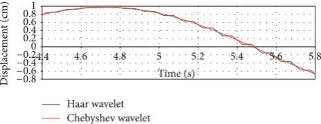
(39) Here𝐼denotes2𝑀-dimensional identity matrix. Finally, substituting(38)and(39)into(36)and(37)vectors of accel-eration, velocity, and displacement being calculated in each collocation point. A schematic view of results calculated with Haar wavelet is depicted inFigure 1. This figure shows a stairs-shaped plot for responses corresponding to all collocation points of Haar wavelet.

3.2. Chebyshev Wavelet. A linear dynamic system can be expressed as

𝑚∗ ̈𝑢 (𝑡) + 𝑐∗ ̇𝑢 (𝑡) + 𝑘∗𝑢 (𝑡) = 𝐹 (𝑡) . (40)

According to(19)accelerations are numerically approxi-mated with Chebyshev wavelet as follows:

̈𝑢 (𝑡) = 𝐶𝑇× 𝜓 (𝑡) . (41)

Vector of velocity is therefore approximated multiplying by operation of integration (𝑃), as follows:

̇𝑢 (𝑡) = 𝐶𝑇_{× 𝑃 × 𝜓 (𝑡) +}_V

𝑛. (42)

Next, displacements are numerically expanded as well as the following:

𝑢 (𝑡) = 𝐶𝑇× 𝑃2× 𝜓 (𝑡) + 𝑢𝑛, (43)

where, in(42)and(43),V𝑛and𝑢𝑛represent initial condition of each global time, approximated with Chebyshev wavelet as a constant value. For this purpose, the unity is being expanded by the Chebyshev wavelet as [25]

1 ≅ 𝐼∗× 𝜓 (𝑡)

≅ (√𝜋

2 ) × [1, 0, 0, . . . , 1, 0, 0, . . .] × 𝜓 (𝑡) .

(44)

Therefore, initial displacements and velocities are improved as

V_𝑛= 𝑆𝑇₁ × 𝜓 (𝑡) ,

𝑢_𝑛= 𝑆𝑇

2 × 𝜓 (𝑡) ,

(6)

where𝑆𝑇₁ and𝑆𝑇₂ are2𝑘−1𝑀 × 1dimension vectors that are obtained by Chebyshev wavelet as follows:

𝑆𝑇₁ ≅V_𝑛(0)× (√𝜋

2 ) × [1, 0, 0, . . . , 1, 0, 0, . . .]𝑇,

𝑆𝑇₂ ≅ 𝑢_𝑛(0)× (√𝜋

2 ) × [1, 0, 0, . . . , 1, 0, 0, . . .]𝑇.

(46)

Substituting (45)into(42)and (43), vectors of velocity and displacement are defined as

̇𝑢 (𝑡) = 𝐶𝑇× 𝑃 × 𝜓 (𝑡) + 𝑆𝑇₁ × 𝜓 (𝑡) ,

𝑢 (𝑡) = 𝐶𝑇× 𝑃2× 𝜓 (𝑡) + 𝑆𝑇1 × 𝑃 × 𝜓 (𝑡) + 𝑆2𝑇× 𝜓 (𝑡) .

(47)

Additionally, external excitation is approximated with Chebyshev wavelet as

𝐹 (𝑡) = 𝑓𝑇× 𝜓 (𝑡) . (48)

Equivalently, the coefficient matrix of load is numerically obtained by

𝑓_1×2𝑇 𝑘−1_𝑀= 𝐹1×2

𝑘−1_𝑀

𝜙₍₂𝑘−1_𝑀)×(2𝑘−1_𝑀). (49)

Furthermore, quantities of dynamic system are modified corresponding on local times as

̇𝑢 (𝑡) = 𝑑𝑡⋅V,

̈𝑢 (𝑡) = 𝑑𝑡⋅ 𝐹 (𝑡𝑛+ 𝑑𝑡⋅ 𝜏, 𝑢,V) .

(50)

Finally, rearranging (40), after algebraic simplifications the dynamic equilibrium is numerically developed as follow-ing algebraic system:

𝑚∗⋅ [𝐶𝑇] + 𝑐∗⋅ 𝑑_𝑡⋅ [𝐶𝑇𝑃 + 𝑆𝑇₁]

+ 𝑘∗⋅ 𝑑2_𝑡⋅ [𝐶𝑇𝑃2+ 𝑆₁𝑇𝑃 + 𝑆𝑇₂] = 𝑓𝑇𝑑2_𝑡. (51)

Equation(51)represents an algebraic system, calculating

𝐶𝑇 _{and substituting into}₍₄₂₎_and ₍₄₃₎_{, displacements and} velocities are obtained at any time instant, respectively.

A schematic view of responses computed with Chebyshev wavelet is depicted in Figure 1. This figure shows a linear plot for responses corresponding to all collocation points of Chebyshev wavelet.

4. Stability Analysis

In general, displacements, velocities, and accelerations have been transferred step-by-step from𝑡th step to the (𝑡 + Δ𝑡)th step of integration schemes. In other words, the relation between quantities from previous state to the current state is expressed as follows [25]:

{̂𝑈_𝑡+Δ𝑡} = [𝐴] {̂𝑈_𝑡} + [𝐿] { ̂𝑓_𝑡+𝜐} , (52)

where, in(52),̂𝑈_𝑡+Δ𝑡represents solution quantities that have been transferred with amplification matrix of𝐴from those on the previous step of𝑈̂_𝑡;𝐿is load operators to relate external load𝑓̂_𝑡+𝜐to the current quantities, known as𝑈̂_𝑡+Δ𝑡;𝜐stands on coefficient ofΔ𝑡and may be 0,Δ𝑡or𝜃Δ𝑡related to each numerical integration method.

To determine the stability criterion of the proposed scheme for Haar wavelet, the behavior of numerical inte-gration should be examined for any initial conditions. For this purpose, the dynamic equilibrium governing on a free vibrated SDOF system in(40)is evaluated. Accordingly,(40) is rearranged in terms of damping ratio (𝜉) and natural frequency (𝜔) as

̈𝑢 (𝑡) + 2𝜉𝜔 ̇𝑢 (𝑡) + 𝜔2_{𝑢 (𝑡) = 0.} ₍₅₃₎

Equation(39)and therefore(38)are rearranged for the initial velocity(V𝑛= ̇𝑢𝑡−Δ𝑡)as follows:

𝑏 = ̇𝑢𝑡−Δ𝑡(𝜅𝜇−1) ,

𝑎 = ̇𝑢𝑡−Δ𝑡𝜂, (54)

where

𝜅 = −𝜔2_{(Δ𝑡) 𝑌 − 2𝜉𝜔 (Δ𝑡) 𝑌 − 𝜔}2_(Δ𝑡)2_𝑌𝑃,

𝜇 = 2𝜉𝜔 (Δ𝑡) 𝑃 + 𝐼 + 𝜔2(Δ𝑡)2𝑃2,

𝜂 = (Δ𝑡) 𝜅𝜇−1𝑃 + (Δ𝑡) 𝑌.

(55)

Note that 𝜇 and 𝐼 (identity matrix) are 2𝑀 × 2𝑀 -dimensional matrix;𝜅and𝜂are1 × 2𝑀-dimensional vectors, respectively. Equivalently, (52) when no load is applied (𝑓̂_𝑡+𝜐= 0) is developed as

[ [

̈𝑢

𝑡

̇𝑢

𝑡

𝑢𝑡]

] = [

[

0 𝑑󸀠_{+ 𝑒}󸀠 _𝑐󸀠

0 𝑎󸀠 ₀

0 𝑏󸀠 _𝑔󸀠]

] [ [

̈𝑢𝑡−Δ𝑡

̇𝑢𝑡−Δ𝑡

𝑢𝑡−Δ𝑡

] ]

. (56)

As it is shown in Figure 1, Haar wavelet functions calculate constant responses on all 2𝑀collocation points. Consequently, components of amplification matrix of 𝐴 computed in(56)represent mean value of2𝑀points in each time interval and we have

𝑎󸀠=mean(𝜅𝜇−1𝑃𝐻_(𝑡)+ 𝐸) ,

𝑏󸀠=mean(𝜂𝑃𝐻_(𝑡)) ,

𝑔󸀠=mean(𝐸) = 1,

𝑑󸀠=mean(−2𝜉𝜔 (𝜅𝜇−1𝑃𝐻_(𝑡)+ 𝐸)) ,

𝑒󸀠=mean(−𝜂𝑃𝐻_(𝑡)𝜔2) ,

𝑐󸀠=mean(−𝐸𝜔2) .

(57)

(7)

0 0.2 0.4 0.6 0.81

4.4 4.6 4.8 5 5.2 5.4 5.6 5.8

Disp

lacemen

t (cm)

Time (s)

Haar wavelet Chebyshev wavelet

−0.2

[image:7.600.55.287.74.164.2]

−0.4 −0.6 −0.8

Figure 1: A schematic view of results calculated with wavelet functions.

from initial accelerations. Although, the same behavior is reported for Chebyshev wavelet [25], the amplification matrix of𝐴and(52)is modified for Chebyshev wavelet in order to be dependent on initial accelerations as

[ [ [ [

...

𝑥𝑡

̈𝑥

𝑡

̇𝑥

𝑡

𝑥𝑡

] ] ] ]

=[[_[

[

0 𝑎𝜙 (𝑡) 𝑏𝜙 (𝑡) 𝑐𝜙 (𝑡) 0 𝑑𝜙 (𝑡) 𝑒𝜙 (𝑡) 𝑓𝜙 (𝑡) 0 𝑔𝜙 (𝑡) 𝑖𝜙 (𝑡) 𝑗𝜙 (𝑡) 0 𝑞𝜙 (𝑡) 𝑟𝜙 (𝑡) 𝑧𝜙 (𝑡) ] ] ] ]

[ [ [ [

...

𝑥𝑡−Δ𝑡

̈𝑥

𝑡−Δ𝑡

̇𝑥

𝑡−Δ𝑡

𝑥𝑡−Δ𝑡

] ] ] ]

, (58)

where

𝑎 = 𝜅𝜇−1_,

𝑏 = 𝜂𝜇−1,

𝑐 = Υ𝜇−1,

𝑑 = 𝐼∗+ 𝜅𝜇−1𝑃,

𝑒 = 𝜂𝜇−1𝑃,

𝑓 = Υ𝜇−1𝑃,

𝑔 = 𝐼∗𝑃 + 𝜅𝜇−1𝑃2,

𝑖 = 𝐼∗+ 𝜂𝜇−1𝑃2,

𝑗 = Υ𝜇−1𝑃2,

𝑞 = 𝐼∗𝑃2+ 𝜅𝜇−1𝑃3,

𝑟 = 𝐼∗𝑃 + 𝜂𝜇−1𝑃3,

𝑧 = 𝐼∗+ Υ𝜇−1𝑃3,

(59)

where

𝜅 = −𝐼∗− 2𝜉𝜔 (Δ𝑡) 𝐼∗𝑃 − 𝜔2(Δ𝑡)2𝐼∗𝑃2,

𝜂 = −2𝜉𝜔 (Δ𝑡) 𝐼∗− 𝜔2(Δ𝑡)2𝐼∗𝑃,

Υ = −𝜔2(Δ𝑡)2𝐼∗,

𝜇 = 𝑃 + 2𝜉𝜔 (Δ𝑡) 𝑃2+ 𝜔2(Δ𝑡)2𝑃3,

(60)

where𝜙(𝑡)denotes2𝑀 × 2𝑀-dimensional coefficient matrix of Chebyshev wavelet.𝐼∗ and 𝑃imply (44) and operation

0 1 2 3 4 5

0 0.25 0.5 0.75 1 1.25 1.5 1.75 2 2.25 2.5

Sp

ec

tral radi

us

Linear acceleration

Average acceleration Central difference

Chebyshev wavelet

Haar wavelet

Wilson(𝜃 = 1.4)

[image:7.600.316.541.74.169.2]

Δt/T

Figure 2: Comparison of spectral radius for proposed methods and 4 other integration schemes.

matrix of integration of Chebyshev wavelet. Note that𝜇 is

2𝑀 × 2𝑀-dimensional matrix; 𝜅, 𝜂, and Υ are 1 × 2𝑀

-dimensional vectors, respectively. The spectral decomposi-tion of 𝐴 = [Φ][𝜆][Φ]−1 is considered for stability and

[Φ]contains eigenvectors of𝐴and[𝜆]is a diagonal matrix including eigenvalues of𝐴. In the pursuit of stable solution the spectral radius of𝐴that equaled by maximum norm of elements[𝜆]should be less than unity as follows [5]:

𝜌 (𝐴) =max(󵄩󵄩󵄩󵄩𝜆₁󵄩󵄩󵄩󵄩,󵄩󵄩󵄩󵄩𝜆₂󵄩󵄩󵄩󵄩,󵄩󵄩󵄩󵄩𝜆₃󵄩󵄩󵄩󵄩) ≤ 1, (61)

where𝜌(𝐴)is the spectral radius of the amplification matrix

𝐴 computed as a function of Δ𝑡 by (56) for the solver of Haar or (58) for the Chebyshev wavelet. This value is calculated for some integration schemes, including,

Wilson-𝜃, central difference, Newmark-𝛽(both linear and average acceleration integration procedure), and the second scale (the least scale) of Chebyshev and Haar wavelet. Results that have been plotted in Figure 2 based on 𝜉 = 0 show that the central difference method and linear acceleration method, as two explicit methods, are conditionally stable whereas the proposed scheme for simple Haar wavelet or complex Chebyshev wavelet is unconditionally stable even in the first two scales of corresponding wavelets. Therefore, no restraints (such asΔ𝑡critical value) are placed on time stepΔ𝑡used in the analysis from the viewpoint of numerical stability considerations.

As it is shown in Figure 2, variation of spectral radius in terms of variation of Δ𝑡/𝑇illustrates that Wilson-𝜃 and average acceleration method are also unconditionally stable with no requirements made on the time stepΔ𝑡used in the analysis.

5. Numerical Applications

(8)

c

F(t) m

IPB300

k

100 300

0 5 10 15 20 25 30

F(t)

Time (s)

F(t) = 300sin(2_{t) N,}moment of inertia IPB_{300 = 25170}cm4

E = 210GPa, mass= 4000kg,𝜉 = 5%, k = 200N/cm,L = 350cm

−100

−300

Figure 3: A fixed beam under sinusoidal loading𝐹(𝑡)applied in vertical direction.

0 0.05 0.1

0 1 2 3 4 5 6 7 8 9 10

Disp

lacemen

t (cm)

Time (s)

Duhamel HA(2M4)

CH(2M4) HA(2M64)

−0.05

[image:8.600.73.522.72.189.2]

−0.1

Figure 4: The first 10 sec of vertical displacement of the mid node (HA = Haar wavelet, CH = Chebyshev wavelet).

0.34

26.03

0.007 0.98 0

0 10 20 30

0 10 20 30 40

CH(2M4) HA(2M4) CH(2M64) HA(2M64) Duhamel

[image:8.600.52.289.238.326.2]

Time consumption Total average errors (%)

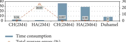
Figure 5: Computation time involved (sec) and percentile total average error for proposed methods (HA = Haar wavelet, CH = Chebyshev wavelet).

recorded with the same hardware. Similarly, for nonlinear analysis of structures recessive proceeding is developed; that is, provisions in the previous step are new initial conditions in the current step for each nonlinear behavior such as stiffness or damping of structure.

5.1. A Fixed Beam. Figure 3shows a fixed I-shaped beam

under sinusoidal loading at the center. The characteristics of considered system including section, mass, dynamic loading, damping ratio, and spring stiffness are shown in this figure. It should be noted that all degrees of freedom are neglected except vertical displacement of the center node.

The first 10 sec time history displacement of the center node is plotted in Figure 4, calculated using the proposed methods of Haar (2𝑀4and2𝑀64) and Chebyshev wavelet (2𝑀4), and compared with results of Duhamel method.

[image:8.600.311.549.263.377.2]

It can be seen from figure that accurate results are calculated by 4th scale of Chebyshev wavelet and 64th Haar wavelet. Significantly, this figure shows that result computed

Table 1: Absolute errors and calculation time of free-scaled Cheby-shev wavelet and Duhamel (example 5.1).

Chebyshev wavelet Duhamel

SM point (Δ𝑡= 0.05 s) (Δ𝑡= 0.01 s)

Δ𝑒 𝑡(sec) 𝑡(sec)

2𝑀= 4 3.40𝐸 − 03 2.8654

8.527

2𝑀= 8 8.91𝐸 − 04 5.3475

2𝑀= 32 1.76𝐸 − 04 9.3321

2𝑀= 64 7.32𝐸 − 05 36.3918

2𝑀= 128 8.00𝐸 − 05 78.8623

2𝑀= 256 8.23𝐸 − 06 141.1936

[image:8.600.63.279.379.452.2]

by 4th scale of Haar wavelet is almost rejected but from its optimization point of view we still accept result of Haar wavelet. In addition, absolute errors and computational times due to the free scale of Chebyshev wavelet consist of 4th, 8th, 32nd,. . ., 256th against Duhamel method is tabulated in Table 1for 10 seconds of loading. It is pointed out that the long interval ofΔ𝑡 = 0.05s and short time step ofΔ𝑡 = 0.01s have been utilized for time increment of wavelet solver and Duhamel scheme, respectively.

Table 1 confirms that high scales of Chebyshev wavelet analyze lateral loading more accurately than low scales. However, computational time gave the maximum value of 141.19 s. Furthermore, it is shown inTable 1that after 64th scale of Chebyshev wavelet accuracy of responses roughly remained constant. However, cost of analysis is considerably increased from the low scales to high scales of Chebyshev wavelet. For the purpose of comparison, percentile errors and computational times have been plotted inFigure 5for two different scales of Haar and Chebyshev wavelet compared with Duhamel integration method.

(9)

0.3 0.8

0 2 4 6 8 10

A

ccelera

tio

n

(g)

Time (s)

−0.2

−0.7

−1.2 S(t)

2IPB240

Ib= ∞

m = 3000kg

[image:9.600.100.505.75.182.2]

𝜉 = 5%, E = 210GPa

Figure 6: A SDOF system subjected to the El-Centro acceleration at the base.

wavelet. Overall, Duhamel results compared with responses of low scale of Chebyshev wavelet demonstrate the efficiency of this basis wavelet even for the low scale of2𝑀 = 4with the least cost of computation, albeit high-scaled Chebyshev wavelet analyzes the lateral loading, accurately.

5.2. A Nonlinear SDOF System Subjected to the Ground

Acceleration. Figure 6shows a SDOF system subjected to

El-Centro acceleration. The characteristics of considered system including two 4 m column’s section, mass, damping ratio, and ground acceleration are shown in this figure. Nonlinearly dynamic analysis is carried out and it is assumed that the nonlinear stiffness (𝑘∗) is defined in term of displacement as

𝑘∗= 4000

√𝑎𝑏𝑠𝑢 + 1. (62)

Nonlinear time history horizontal displacement of the considered mass using Chebyshev and Haar wavelet for time increment ofΔ𝑡 = 0.05sec compared with Wilson-𝜃method

forΔ𝑡 = 0.05and 0.001 sec is plotted inFigure 7. It is shown

in the figure that results computed even with low scale of Haar wavelet are closer than results calculated for a large time increment of Wilson-𝜃. In addition, this figure illustrates high accuracy of low-scaled Chebyshev wavelet and large-scaled Haar wavelet in comparison with long time increment of Wilson-𝜃method.

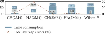
Furthermore, computation time involved and percentile total average errors are plotted in Figure 8 for proposed schemes and Wilson-𝜃method. For the purpose of compari-son, time history responses calculated with Wilson-𝜃method with time increment of Δ𝑡 = 0.001sec are supposed as exact results and errors are presented compared with exact responses.

Considerably, Figure 8illustrates that optimal dynamic analysis has been achieved by 4th scale of Chebyshev wavelet. Significantly, cost of analysis is reduced by 6.98 sec and accuracy of 2.97% of errors. Moreover, Figure 8 shows an inefficient nonlinear analysis for Haar wavelet, particularly encountering with broad-frequency-content excitation (El-Centro acceleration shown inFigure 6). Imprecise approx-imation of high frequency components by Haar wavelet and using an alternative solver significantly affects the cost of analysis. Consequently, the applicability of the proposed approaches is demonstrated by given numerical examples, in which that the linear and nonlinear time history analysis of

0.01 0.03 0.05

0 1 2 3 4 5 6 7 8 9 10

Disp

lacemen

t (cm)

Time (s)

CH(2M4) HA(2M4)

HA(2M64)

−0.01

−0.03 −0.05

Wilson-𝜃(Δt = 0.001)

[image:9.600.312.545.231.321.2]

Wilson-𝜃(Δt = 0.05)

Figure 7: The first 10 sec horizontal displacement of the SDOF system (HA = Haar wavelet, CH = Chebyshev wavelet).

2.97

38.03

0.063 3.01

3.21 6.98

57.77 48.23

63.02

0

0 20 40

0 50 100

CH(2M4) HA(2M4) CH(2M64) HA(2M64)

Time consumption Total average errors (%)

Wilson-𝜃

Figure 8: Computation time involved (sec) and percentile total average error for proposed methods; HA = Haar wavelet, CH = Chebyshev wavelet (Δ𝑡 = 0.05); Wilson-𝜃(Δ𝑡 = 0.001).

the smooth parts and broadband frequency contents of the external loading are optimally accomplished using moderate scales of the simple Haar and low scales of the complex Chebyshev wavelets, respectively.

6. Conclusion

[image:9.600.321.538.373.444.2]

(10)

implemented, therefore evaluation of the equation of motion is optimally achieved. In other words, an adaptive numerical scheme has been developed to be capable of capturing details in the vicinity of highly varying structural responses. Eventually, it is demonstrated that the proposed methods for both wavelet functions lie on unconditional stable methods.

Despite accurate responses for large scales of Chebyshev wavelet due to the inherent ability of this wavelet, the opti-mum results were computed using its low-scaled functions. In actual fact, practice of several basis functions in the proposed approach, yielding an adaptive wavelet approach, varies from cases to cases. Consequently, compatible analysis is satisfied using 2D and simple functions to analyze the smooth parts of loading and employing 3D and complex wavelet functions to analyze wide-frequency-contents parts, simultaneously. It is recommended to employ the proposed methods for the solution of optimization problems, where the objective functions of dynamic equilibrium governing to the large-scaled structural systems are considered for satisfaction of various constraints.

Conflict of Interests

The authors declare that there is no conflict of interests regarding the publication of this paper.

Acknowledgments

The authors wish to acknowledge the financial support from the University of Malaya (UM) and Ministry of Education of Malaysia (Grant nos. PG078/2013B and UM.C/625/1/HIR /MOHE/ENG/55).

References

[1] K. J. Bathe,Finite Element Procedures, Prentice-Hall, Englewood Cliffs, NJ, USA, 1996.

[2] T. J. Hughes, The Finite Element Method, Linear Static and Dynamic Finite Element Analysis, Prentice-Hall, Englewood Cliffs, NJ, USA, 1987.

[3] A. K. Chopra,Dynamic of Structures: Theory and Applications to Earthquake Engineering, Prentice Hall, Englewood Cliffs, NJ, USA, 1995.

[4] M. A. Dokainish and K. Subbaraj, “A survey of direct time-integration methods in computational structural dynamics. I. Explicit methods,”Computers & Structures, vol. 32, no. 6, pp. 1371–1386, 1989.

[5] K. J. Bathe and E. L. Wilson, “Stability and accuracy analysis of direct integration methods,”International Journal of Earthquake Engineering and Structural Dynamics, vol. 1, no. 3, pp. 283–291, 1972.

[6] S.-Y. Chang, “Explicit pseudodynamic algorithm with uncon-ditional stability,”Journal of Engineering Mechanics, vol. 128, no. 9, pp. 935–947, 2002.

[7] G. Rio, A. Soive, and V. Grolleau, “Comparative study of numerical explicit time integration algorithms,”Advances in Engineering Software, vol. 36, no. 4, pp. 252–265, 2005. [8] C. F. Chen and C. H. Hsiao, “Wavelet approach to optimizing

dynamic system,”IEE Proceedings—Control Theory and Appli-cations, vol. 146, no. 2, pp. 213–219, 1999.

[9] T. Fang, X. L. Leng, and C. Q. Song, “Chebyshev polynomial approximation for dynamical response problem of random system,”Journal of Sound and Vibration, vol. 266, no. 1, pp. 198– 206, 2003.

[10] E. Salajegheh and A. Heidari, “Time history dynamic analysis of structures using filter banks and wavelet transforms,” Com-puters and Structures, vol. 83, no. 1, pp. 53–68, 2005.

[11] S. H. Mahdavi and H. A. Razak, “Optimum dynamic analysis of 2D frames using free-scaled wavelet functions,”Latin American Journal of Solids and Structures, vol. 11, no. 6, pp. 1036–1048, 2014.

[12] N. Chen, Z. Qian, and X. Meng, “Multistep wind speed fore-casting based on wavelet and gaussian processes,”Mathematical Problems in Engineering, vol. 2013, Article ID 461983, 8 pages, 2013.

[13] C. Cattani, “Haar wavelets based technique in evolution prob-lems,”Proceedings of the Estonian Academy of Sciences, Physics, Mathematics, vol. 53, no. 1, pp. 45–63, 2004.

[14] L. A. D´ıaz, M. T. Mart´ın, and V. Vampa, “Daubechies wavelet beam and plate finite elements,”Finite Elements in Analysis and Design, vol. 45, no. 3, pp. 200–209, 2009.

[15] S. U. Islam, I. Aziz, and F. Haq, “A comparative study of numerical integration based on Haar wavelets and hybrid functions,”Computers & Mathematics with Applications, vol. 59, no. 6, pp. 2026–2036, 2010.

[16] S. H. Mahdavi and S. Shojaee, “Optimum time history analysis of SDOF structures using free scale of Haar wavelet,”Structural Engineering and Mechanics, vol. 45, no. 1, pp. 95–110, 2013. [17] U. Lepik, “Haar wavelet method for solving stiff differential

equations,”International Journal of Mathematics and Computa-tion, vol. 14, no. 1, pp. 467–481, 2009.

[18] ¨U. Lepik, “Numerical solution of differential equations using Haar wavelets,”Mathematics and Computers in Simulation, vol. 68, no. 2, pp. 127–143, 2005.

[19] E. Babolian and F. Fattahzadeh, “Numerical computation method in solving integral equations by using Chebyshev wavelet operational matrix of integration,”Applied Mathematics and Computation, vol. 188, no. 1, pp. 1016–1022, 2007.

[20] L. Fox and I. B. Parker,Chebyshev Polynomials in Numerical Analysis, Oxford University Press, London, UK, 1968. [21] J. C. Mason and D. C. Handscomb, Chebyshev Polynomials,

Chapman & Hall/CRC, 2003.

[22] E. Babolian and F. Fattahzadeh, “Numerical solution of differ-ential equations by using Chebyshev wavelet operational matrix of integration,”Applied Mathematics and Computation, vol. 188, no. 1, pp. 417–426, 2007.

[23] M. Ghasemi and M. T. Kajani, “Numerical solution of time-varying delay systems by Chebyshev wavelets,”Applied Math-ematical Modelling, vol. 35, no. 11, pp. 5235–5244, 2011. [24] Y. Li, “Solving a nonlinear fractional differential equation using

Chebyshev wavelets,”Communications in Nonlinear Science and Numerical Simulation, vol. 15, no. 9, pp. 2284–2292, 2010. [25] S. H. Mahdavi and H. Abdul Razak, “A wavelet-based approach

(11)

Submit your manuscripts at

http://www.hindawi.com

Hindawi Publishing Corporation

http://www.hindawi.com Volume 2014

Mathematics

Journal of

Mathematical Problems in Engineering

Hindawi Publishing Corporation http://www.hindawi.com

Differential Equations

International Journal of

Volume 2014

http://www.hindawi.com Volume 2014 Hindawi Publishing Corporationhttp://www.hindawi.com Volume 2014

Mathematical PhysicsAdvances in

Complex Analysis

Journal of

Optimization

Journal of

Combinatorics

International Journal of

Journal of

Function Spaces

Abstract and Applied Analysis

International Journal of Mathematics and Mathematical Sciences

Hindawi Publishing Corporation http://www.hindawi.com Volume 2014

The Scientific

World Journal

Discrete Dynamics in Nature and Society

http://www.hindawi.com Volume 2014 Hindawi Publishing Corporation

Discrete Mathematics

Journal of