Continued Fractions and Dynamics

http://dx.doi.org/10.4236/am.2014.57101

How to cite this paper: Isola, S. (2014) Continued Fractions and Dynamics. Applied Mathematics, 5, 1067-1090. http://dx.doi.org/10.4236/am.2014.57101

Continued Fractions and Dynamics

Stefano Isola

Dipartimento di Matematica e Informatica, Università degli Studi di Camerino,Camerino Macerata, Italy Email: [email protected]

Received 17 January 2014; revised 17 February 2014; accepted 24 February 2014

Copyright © 2014 by author and Scientific Research Publishing Inc.

This work is licensed under the Creative Commons Attribution International License (CC BY).

http://creativecommons.org/licenses/by/4.0/

Abstract

Several links between continued fractions and classical and less classical constructions in dynam-ical systems theory are presented and discussed.

Keywords

Continued Fractions, Fast and Slow Convergents, Irrational Rotations, Farey and Gauss Maps, Transfer Operator, Thermodynamic Formalism

1. Introduction

The connection between Number Theory and Dynamical Systems Theory is receiving recently a considerable attention. In this paper, we review some aspects of this connection focusing on the interplay between continued fractions and one dimensional dynamics. In Section 2, we review some known facts about fast and slow con-vergents, highlighting their relations both with irrational rotation dynamics and the ergodic theory of the Gauss map. In Section 3, after recalling the construction and the basic properties of the Farey tree, we describe differ-ent ways of coding the paths on it, as well as their dynamical counterparts obtained by combining fractional li-near transformations. Deeper insights into these connections are provided by the Minkowski question mark function, whose properties are discussed in Section 4. Finally, in Section 5, we present some applications of the thermodynamical formalism based on the previous constructions.

2. Fast and Slow Convergents

We start by reviewing some well known facts about continued fractions1. Let

[

1 2 3

]

1

2 3 1

, , , 1

1

x a a a

a a

a

= ≡

+ +

+





(2.1)

be the continued fraction expansion of the number x∈

[ ]

0,1 . By applying Euclid’s algorithm one sees that the above expansion terminates if and only if x is a rational number. For x irrational one can construct recursively a sequence p_n q_n of rational approximants of x as

1 1 1

0 0 1 1

1 1 1 1

0 1

, and , 1

1

n n n n n n n n

p a p p

p q p q n

a q a q q

+ + −

+ + −

+

= = = ≥

+ (2.2)

We can write this recursion in matrix form as follows: letting

1 0 1 1

: and :

1 1 1 0

A =_ _ B =_ _

    (2.3) and noting that

1 1

1 0 k k

BA − =  _

  (2.4) we have

1

1 0

1 0

a

p p

A

q q

 

=

 

  (2.5) and

1 1 2

1 1 1

1

, 1

n

n n a a a

n n

p p

A BA BA n

q q

+

+ − −

+

 

= ≥

 

   (2.6)

A short manipulation of (2.2) gives q_n+1p_n−q p_{n n+1}= −

(

q p_{n n−1}−q_n−1p_n

)

. Since q p_{1 0}−q p_{0 1}= −1 one ob- tains inductively the Lagrange formula

( )

1 1 1 , 1.

n n n n n

q p₋ −q₋ p = − n≥ (2.7) Another useful formula which can be easily obtained from (2.2) is the following: for all

r

≥

1

and n≥1,

1 1 2 3

1 1

, , , , n n

n

n n

rp p

a a a a

r rq q

−

−

+

 ₊ _{= ⋅}

  ₊

   (2.8)

Letting r→ ∞ we get in particular

[

1, 2, ,

]

n n

n

p

a a a

q

= ⋅

 (2.9)

Note that

1

2

1 3 1

2

1 1

1 1

1 n

n

n n

n

n n n

n

q

q _{a a}

q

a q q

q

−

−

− − −

−

= =

+ +

+

and so forth. We thus have the so called mirror formula (some consequences of which have been investigated in [4]):

[

]

1

[

]

1 2 1 1

If n , , , then n , , ,

n n n

n n

p q

a a a a a a

q q

−

−

1069 The numbers n

n

p

q are called continued fraction convergents (CFC) of x and it turns out that the n-th CFC

n n

p

q is the best rational approximation to

x

whose denominator does not exceed qn [2]. One sees that

2 2 1

2 2 1

, 0.

n n

n n

p p

x n

q q

−

−

< < ∀ > (2.11)

Putting r=a_n+₁ in (2.8) we get

[

]

1

1 2 3 1 2 3 1

1 1

1

, , , , , , , , , n

n n n

n n

p

a a a a a a a a a

a q

+ +

+ +

 

+ ≡ = ⋅

 

    (2.12)

But what happens if r in (2.8) takes on an intermediate value 1, 2,,an+₁?

Definition 2.1 For n≥1 the sets 1 1

n n n n

rp p rq q −

−

 + 

 ₊ 

  for 1≤ ≤r an+1 are the n’th Farey convergents (FC) for the real number x∈

[

0,1

)

.

Example. Let x= − =e 2

[

1, 2,1,1, 4,1,1, 6,

]

. The first five CFC are

1 1

1 p 1

n

q

= =

2 2

1 2

2

1 3

1 2

p n

q

= = =

+

3

3

1 3

3

1 4

1 1 2

1

p n

q

= = =

+ +

4 4

1 5

4

1 7

1

1 2

1 1

1

p n

q

= = =

+ +

+

5

5 1 23

5

1 32

1

1 2

1 1

1 1

4

n

q

= = =

+ +

+ +

On the other hand, within the same accuracy, there are 2 1 1 4+ + + =8 FC’s. They are

1,1 1 0

1,1 1 0

1 1, 1,

2

t p p

n r

s q q

+

= = = =

+

1,2 1 0

1,2 1 0

2 2

1, 2,

2 3

t p p

n r

s q q

+

= = = =

+

2,1 2 1

2,1 2 1

3 2, 1,

4

t p p

n r

s q q

+

= = = =

1070

3,1 3 2

3,1 3 2

5 3, 1,

7

t p p

n r

s q q

+

= = = =

+

4,1 4 3

4,1 4 3

8 4, 1,

11

t p p

n r

s q q

+

= = = =

+

4,2 4 3

4,2 4 3

2 13

4, 2,

2 18

t p p

n r

s q q

+

= = = =

+

4,3 4 3

4,3 4 3

3 18

4, 3,

3 25

t p p

n r

s q q

+

= = = =

+

4,4 4 3

4,4 4 3

4 23

4, 4,

4 32

t p p

n r

s q q

+

= = = =

+

We now need some notions.

Definition 2.2 The Farey sum over two rationals a

b and a b

′

′ is the mediant operation given by

:

a a a a a

b b b b b

′ + ′ ′′

⊕ = = ⋅

′ + ′ ′′ (2.13) It is easy to see that a

b

′′

′′ falls in the interval , a a b b

′

 

 _′

 

2_{. We say that} a

b and a b

′

′ are Farey neighbours if

1

ab′−a b′ = ± . Two Farey neighbours define a Farey interval and each Farey interval can be labeled uniquely according to the mediant (child) a a a

b b b

′′₌ + ′

′′ + ′ of the neighbours.

Observe that given a pair of consecutive FC’s, say

(

)

(

)

, 1 , 1 1

, 1 , 1 1

1 and

1

n r n n n r n n

n r n n n r n n

t rp p t r p p

s rq q s r q q

+ −

−

− + −

+ +

+

= =

+ + +

for some n≥1 and 1≤ <r an+₁, we have

, 1 ,

, 1 ,

n r n r n

n r n r n

t t p

s s q

+

+

= ⊕ ⋅ (2.14) Moreover

( )

, , 1 1

1 n

n n n n

n r n r n n

q p q p

t −s = p₋ −q ₋ = − (2.15)

by Lagrange’s formula. Therefore, for every n≥1, each FC , , n r

n r

t

s for r=1,,an+1 is a Farey neighbour of

n n

p

q , the corresponding Farey interval getting smaller and smaller as r increases. More precisely, using again Lagrange’s formula, one easily obtains

(

)

1

1 1

1

n n n

n n n n n n

p rp p

q rq q q rq q

−

− −

+

− = ⋅

+ + (2.16)

We therefore see that the FC , , n r

n r

t

s is the best one-sided rational approximation to x whose denominator

2

1071

does not exceed s_{n r,} (although, if r<a_n+₁, there might be a CFC with denominator less than sn r, and closer

to

x

on the other side of x). Increasing r, once we arrive at r=a_n+₁ we hit a new CFC on the current side of

x

, closer than the previous CFC. Finally, using matrix notation, the FC’s can be expressed in terms of intermediate products in (2.5) for n≥1 as

1 2

, 1 1 1

1 ,

, 1 .

n

n r n a a a r

n n r n

t p

A BA BA BA r a

s q

−

− −

+

 _{= ≤ ≤}

 

   (2.17)

The algorithm which produces the sequence of FC‘s of a given real number is called slow continued fraction algorithm (see, e.g., [6] [7]).

Remark 2.3 The set





_ of Farey fractions of order



is the set of irreducible fractions in

[ ]

0,1 with de- nominator ≤, listed in order of magnitude (see [8]). Thus, ₁ 0 1,

1 1   = _ _



 ,

2 3 4

0 1 1 0 1 1 2 1 0 1 1 1 2 3 1

, , , , , , , , , , , , , ,

1 2 1 1 3 2 3 1 1 4 3 2 3 4 1

     

=_{ } =_{ } =_{ }

     

  

  

and so on. In particular

( )

2

2 1

3 2

π k=ϕ k − =

∑



 

 _

 with Euler totient function

( )

k

{

0 i k: gcd ,

( )

i k 1

}

ϕ

= < ≤ = . Then we see that each ,

, n r

n r

t

s for r=1,,an+1 is consecutive to

n n

p

q in 



 for s_{n r,} < ≤ s_{n r, +1}.

2.1. Connection to Rotations of the Circle

One can interpret the above construction in terms of a kind of renormalization procedure for rotations of the circle

[

0,1 through an angle

)

x. With no loss we take the initial point to be the origin 0 and set J₀ =

[ ]

0,x . Since 1

1

a x

 

=  _{ } we have a x₁ ≤ <1

(

a₁+1

)

x and thus

1 0 1

1=a J + J

with

1 1 1 1 1.

J = −a x= p −xq (2.18) Moreover we have

[

]

1

1 2 3

0 1

, ,

J

a a a

J = −x = 

and therefore a J_{2 1} ≤ J₀ <

(

a₂+1

)

J₁ or, which is the same,

0 2 1 2

J =a J + J

with

(

)

2 2

1

1 2 2

.

J

= −

x a

−

a x

=

q x

−

p

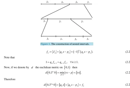
(2.19) Iterating this procedure, we construct a family of nested intervals (see Figure 1) J_n, n≥0, such that

[

1 2

]

1

, , n

n n n

J

a a

J ₋ = + +  (2.20)

and

1 1 1 , 0,

n n n n

[image:6.595.83.530.84.387.2]

Figure 1. The construction of nested intervals.

( ) (

)

: 1n .

n n n n n n

f = J = q x−p = − q x−p (2.22) Note that

1 1

1=q fn n− +qn− fn, ∀ ≥n 1. (2.23)

Now, if we denote by d the euclidean metric on

[

0,1 then

)

(

0, r0

)

min : .

p

d T rx p rx

∈

= − =

 (2.24)

Therefore

(

0, qn0

)

n n n n

d T = q x = q x−p = f (2.25) That is, the sequence of arc-lengths f_n is but the sequence of successive closest distances to the initial point. This can be seen in the following way: starting from 0 and iterating a₁ times one ends up at the point

1 1

a x=q x which lies on the left of 0 and is the point closest to 0 up to now, being distant J1 from it. Iterating 1

a more times one ends up at the point 2a1x=2q1x which lies on the left of 0 at distance 2 J1 , ... iterating 2 1

a a times one ends up at the point

a a x

_{2 1}

=

a q x

_{2 1}

=

(

q

₂

−

1

)

x

which still lies on the left of 0, at distance

2 1

a J

. One more iterate yields the point q x₂ which now lies on the right of 0 at distance

J

₂ and is the point closest to 0 up to now, and so on and so forth (for more details see [9]). The above implies that the first return map in the interval J_n (which is

[

0,f_n

]

or

[

1− f_n,1

]

according whether n is even or odd) is the rotation through the angle

( )

1 1 1 1 1

n

n n n

f q x p

+

+ + +

− = − . Finally, one has the equivalence:

[

1

]

0 , , n

n n

n

p

f x a a

q

≈ ⇔ ≈  = ⋅ (2.26)

In addition, for each r=1,,an+₁, it holds

,

1 1

, 1

, , n r

n n n

n r

t

f f r x a a

r s

−  

≈ ⇔ ≈_ + _= ⋅

   (2.27) The three distance theorem. The points

{ }

kα with 0≤ ≤k  partition the unit circle into



+

1

intervals. A classical result (see e.g. [10]), which can be easily obtained by induction using the above construction, is that the possible lengths of these intervals are organized according to the Farey convergents in the following way: • If 0< ≤ q₁ then there are two distinct lengths: f₀ and 1−f₀ (which become f₀ and f₁ when

1

q

=

 ).

• If rqn+qn−₁≤ < +

(

r 1

)

qn+qn−₁ for some n≥1 and 1≤ ≤r an+1 then there are at most three lengths:

n

f , f_n−1−rf_n and fn−₁− −

(

r 1

)

fn, the last of which disappears when = +

(

r 1

)

qn+qn−1−1.

We point out that in the second case above there are two intervals, chosen from among those having the smallest lengths:

(

) (

)

1 1 1

and

n n n n n n n n n

1073

which have 0 as their common endpoint. We then see that the approximations (26) and (27) are the same as shrinking one of these intervals to zero. Moreover, the fractions n

n

p q and

1 1

n n n n

rp p rq q −

−

+

+ are the two successive

elements of _n having

x

between them (see also Remark 2.3).

2.2. Growth of Denominators

The Gauss map G: 0,1

[ ] [ ]

→ 0,1 is defined as

( ) { }

1 for 0 and

( )

0 0.

G x = x x> G = (2.28) It is well known that G has an a.c. invariant ergodic probability measure µ given by

( )

1

₍

d

₎

d

log 2 1

x x

x

µ =

+ (2.29)

A short reflection shows that 1, 2, ,

( )

n n

x=_a a  a +G x _ or else

( )

(

)

( )

(

)

1

1 1

1

n

n n n

n n

G x p p

x

G x q q

−

− −

−

+

= ⋅

+ (2.30)

From this we obtain at once

( )

1 1 1

,

n n n n

n n n

q x p f

G x

q−x p− f −

−

= − = −

− (2.31)

where the numbers f_n have been introduced in (2.22). Therefore

( )

0 n

k n

k

f G x

= =

∏

and, by the ergodic theorem, we have for µ-almost all x∈

[ ]

0,1 and then almost everywhere,

( )

2

1

0

1 π

lim log log d

12 log 2 n

n→∞_n f =

∫

xµ x = − ⋅ (2.32) Since _

(

Gn

( )

x

)

−1 =_ a_n+₁ and thus

(

( )

)

1

1 1 1

n

n n

a₊ < G x − <a₊ + another consequence of (2.30) is that

1 1 1 1

1 1

2

n n

n n

n n n n n

q q

q f

a + q q+ q + a+

< < < <

+ +

and therefore using (2.31)

1 1

1.

2<q fn n− < (2.33) Putting together (2.32) and (2.33) we get the classical theorem of Lévy

2

log π

almost everywhere 12 log 2

n

q

n →

On the other hand we may expect the growth of FC’s denominator to be subexponential. Indeed, let ,

, n r m

m n r

t t

s ≡s with 2

n k k

m=

∑

₌a +r be the m-th FC. Its denominator satisfies q_n <s_m≤q_n+₁. It is a result of Khinchin and Lévy (see [1]) that

1

1 1

in measure

log log 2

n k k

a n n =

→

Combining the above we get the following

Lemma 2.4

2

log π

in measure 12 log

m

s

m  m

Of course there are special behaviours: take x=

(

5 1 2−

)

=

[

1,1,1,

]

, then s_n =q_n and both are equal to the n-th Fibonacci number. Hence n−1logq_n converge to x−1.

3. A Walk on the Farey Tree

Having fixed



≥

1

, let _ be the ascending sequence of irreducible fractions between 0 and 1 constructed inductively in the following way: set first ₁ 0 1,

1 1   = _ _

 , then _ is obtained from _−1 by inserting among

each pair of neighbours a b and

a b

′

′ in −1 their child a b

′′

′′ as in (2.13). Thus

2 3 4

0 1 1 0 1 1 2 1 0 1 1 2 1 3 2 3 1

, , , , , , , , , , , , , , , ,

1 2 1 1 3 2 3 1 1 4 3 5 2 5 3 4 1

     

=_{ } =_{ } =_{ }

     

  

and so on. The elements of _ are called again Farey fractions. Evidently _ ⊇_.

Remark 3.1 It has been shown in ([11], Thm 2.6) that the set

{

logb

}

a F b

 _∈ 

 

  becomes equidistributed as

→ ∞

 . More specifically, the probability measure _{{ }}

1 log 1

2+1

∑

ab∈+δ b converges to the Lebesgue measure on

[ ]

0,1

.

Definition 3.2 For



≥

1

we say that a Farey fraction

x

has rank



if x∈  +₁ . We also define the rank 0 rank 1 0

1 1

 ₌  ₌    

    . For



≥

1

there are exactly

1

2− Farey fractions of rank



and their sum is equal to 2

2− . Recall that every rational number x∈

( )

0,1 has a unique finite continued fraction expansion x=

[

a₁,,a_n

]

with an >1 [2]. The validity of the following relation will arise straight-

forwardly in the sequel:

Lemma 3.3

[

1

]

( )

1

, , rank 1

n

n i

i

x a a x a

=

=  → =

∑

−

Remark 3.4 Note that, according to the above Lemma, the cardinality ₂−1 _of

1

+

 

   can be interpreted

as the number of choices of integers a₁,,an, with 1≤ ≤n  and so that ai≥1 for i=1,,n−1, an >1

and

∑

ni=₁ai= + 1. Indeed, for each fixed n the number of such choices is

1 1

n

−    ₋   



, then sum over

1, ,

n=  .

It is also easy to realize that all Farey fractions which fall in the interval 1 ,1 1

 

 ₊ 

  have rank greater than or

equal to



+

1

, whereas their continued fraction expansion starts with a₁=.

An interesting object is the Farey tree  whose vertex-set is 

( )

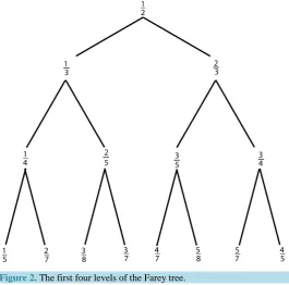
0,1 and which is constructed as follows (see Figure 2):

• every column in  contains one entry (vertex or node); • for



≥

1

the



-th row is   _{+1 };

• the node a a

b b

′ +

′

+ , representing the interval , a a b b

′

 

 _′

 , is connected by edges to its left child

2 2

a a

b b

′ +

′ + and right child 2

2

a a

b b

′ +

′

[image:9.595.181.447.86.348.2]

1075

Figure 2. The first four levels of the Farey tree.

Note that the fractions 0 1 and

1

1 play the role of ancestors when using the Farey sum to obtain one row from the previous one. Besides the Farey sum, an alternative way to construct recursively the entries of  is as follows.

Definition 3.5 Given a

b∈ its descendants are the symmetrical entries of  given by

a a+b and

b a+b, respectively.

Lemma 3.6 The collection of all descendants of the entries of a given row in  is precisely the underlying row.

Proof. If

[

₁, , n

]

a

a a

b =  then

[

1 1, , n

]

a

a a

a+b= +  and

[

1, 1, , n

]

b

a a

a+b=  . Therefore

rank a rank b rank a 1

a b a b b

 ₌  ₌  ₊

 ₊   ₊   

      and the claim follows.

♦

Remark 3.7 If a

[

a a₁, ₂ ,a_n

]

b=  and

[

n, n1, , 1

]

a

a a a

b −

′ =

′  then rank rank

a a

b b

′  ₌      _′

    and b=b′.

3.1. The

{ }

L R

,

Coding

Every rational number in

( )

0,1 appears exactly once in the above construction and corresponds to a unique finite path on  starting at the root node 1

2 and whose number of vertices equals the rank of the rational number. We can code this path in the following way: first, any l

r∈ can be uniquely decomposed as 3

with 1

l m n

ns mt

r= s ⊕t − = (3.1) and the unimodular relations

1

sl−rm=rn− =lt ns−mt= (3.2) plainly hold. The neighbours m

s and n

t are thus the ‘parents’ of

l

r in  and we may accordingly identify

n m

l

t s

r

 

⇔_{ }∈

   (3.3) with

0 , 0 , 1

a b

a c b d ad bc c d

  

 

=  < ≤ ≤ < − = ⋅

  

 

 (3.4)

Note that the left column bears on the right parent and viceversa. Thus 1 0

1

1 1 2

  ⇔  

  (3.5) On the other hand, any l

r as above has a unique pair of (left and right) children, given by

and

m m n m n n

s s t s t t

+ +

⊕ ⊕

+ + (3.6) respectively. In order to generate them we set

1 0 1 1

: and :

1 1 0 1

L =_ _ R =_ _

    (3.7) Note that for k∈

1 0 1

: and :

1 0 1

k k k

L R

k

   

=_{ } =_{ }

    (3.8)

and also

1 0 1

with .

1 0

k k

R S =SL S=S− =  _

  (3.9)

Moreover, we have

1 0 1 1

n m m n m m m n

t s s t s s s t

+

     +

= ⇔ ⊕

    ₊  ₊

     (3.10)

and

1 1 0 1

n m n m n m n n

t s t s t s t t

+

   ₌ _⇔ + _⊕

    ₊  ₊

     (3.11)

In other words, the matrices L and R, when acting from the right, move to the left and right child in , respectively. Moreover, it is plain that given Y∈ we have YR∈ and YL∈. We have thus proved the following

Proposition 3.8 To each entry x∈ there corresponds a unique element X∈ which, in turn, can be uniquely presented as

i i

X =L

∏

M (3.12) where the number of terms in the product _i

i

L

∏

M

is equal to

rank

( )

x

and Mi = L or Mi = R according

whether the i-th turn, along the descending path in  which starts from the root node 1

1077

Remark 3.9 By the way, the matrices L and R induce the so called Farey tesselation of the upper half plane

{

: Im 0

}

H = z z> (see [12]).

Example. 3

10 is the right child of

2

7, which is the right child of 1

4, which is the left child of

1

3, which is

the left child of 1 2. Thus

1 2 3

3 7

10 LLLRR

 

⇔_{ }=

 

For 3

11, which is the left child of

2

7, we find

2 1

3

7 4

11 LLLRL

 

⇔_{ }=

 

Note that rank 3 rank 3 5

10 11

 ₌  ₌

   

    .

To any given irrational number x∈

[ ]

0,1 we may associate a unique infinite path on  , and thus a unique semi-infinite word in

{ }

L R, . Bearing in mind the continued fraction expansion (2.1) of x, let

1,1

1,1 1 1

1

t

s =a +

the first FC of x. In order to reach it from the top of  we need the block _La1−1_{. Whence we code x through} the map

φ

: 0,1

[ ] { }

→ L R,  defined by

( )

1

1 2

a

x L M M

φ =  (3.13) where M_i=L or M_i =R according whether the i-th turn along the infinite path in  which starts from

1,1

1,1

t

s and approaches x along the sequence of successive FC’s goes left or right. This coding is faithful to the

binary structure of  but apparently not so much to the continued fraction expansion of x. To make the latter more transparent we may note that, according to the characterization of the FC’s given above (see (2.15) and (2.16)), the symbols L and R in (3.13) come in blocks whose lengths are given by nothing but the partial quotients a_i of

x

. More precisely, a short reflection shows that the following rule is in force: the first block is such that M_i=R if 1≤ ≤i a₂. Moreover, for k≥2 let

2 ,

k k i

i

b a

=

=

∑

then we have

2 2 2 1

2 1 2

, if ,

, if .

k k

i

k k

L b i b

M

R b i b

− −

−

< ≤ 

=  _{< ≤}



In other words, we have the coding

[

]

( )

1 2 3

1, 2, 3, =

a a a

x= a a a  ↔φ x L R L  (3.14) Furthermore we set φ

( )

0 =L∞ and φ

( )

1 =LR∞. More generally, we note that each rational x has two infinite paths which agree down to node

x

: they are those starting with the finite sequence coding the path to reach x from the root node and terminating with either RL∞ or LR∞. We shall agree that φ

( )

x terminates with RL∞ or LR∞ according whether the number of its (finite) partial quotients is even or odd. On the other hand, for notational simplicity’ sake we shall assume this agreement only implicitly. We summarize the above in the following

que sequence

φ

( ) { }

x ∈ L R,  given by φ

( )

_x =_{L R L}a1 a2 a3 _{which represents an infinite path on}  _whose

sequence of vertices starting from the a₁-th is precisely the sequence

(

t s

_{m m m}

)

_≥1 of FC’s of x. Moreover, if



denotes the lexicographic order on

{ }

L R,  then

( )

( )

.

x> ⇒y

φ

x 

φ

y

An simple consequence of the above construction is the following result.

Proposition 3.11 Let x=

[

a₁,,a_n

]

with an >1 and

n

even. Then its left and right children in  are given by x′ =

[

a₁,,a_n−1, 2

]

and x′′ =

[

a₁,,a_n+1

]

, respectively. If instead

n

is odd the expansions for

x′ and x′′ have to be interchanged. Proof. Since

n

is even we can write

[

]

( )

1 2 1

1, , .

n

a a a n

x= a  a ↔φ x =L R R − (3.15) Therefore

(

1 2 1

)

(

1 2

)

1 a a an _and 1 a a an

x′=φ− L R R −L x′′=φ− L R R

which yield the claim. A similar reasoning applies for n odd. ♦

3.2. The {

A

,

B

} Coding

Using (3.9) we can write

3 3

1 2 a 1 2 a

a a a a

L R L =L SL SL  (3.16) On the other hand we have L≡A and (see (2.4))

1 1

1 0

k k k

SL =_ _=BA−

  (3.17) This defines a recoding

ψ

: 0,1

[ ] { }

→ A B,  so that

[

]

( )

1 2 1 3 1

1, 2, 3,

a a a

x= a a a  ↔ψ x =A BA −BA −  (3.18) The FC , 1

, 1 n r

n r

t

s

+

+

of

x

, which has rank

1

n i i=a r

=

∑

+

 , will then be expressed as

1 2

1 2

, 1

, 1

, odd, , even, n

n a a a r n r

a a a r n r

t L R L R n

s L R R L n

φ +

+ 

 _{ }

=

  

 _{ }

  



 (3.19)

or else

1 2

, 1 1 1 1

, 1

.

n

n r a a a r

n r

t

A BA BA BA

s

ψ + − − −

+

 

=

 

 

   (3.20)

Note that both expansions have exactly



terms and the latter agrees with (2.17) once we interpret the l.h.s. of (2.17) as the FC , 1

, 1 n r

n r

t

s

+

+

of x, that is taking the Farey sum of the columns in the same spirit as (3.3). Example. The example with x= − =e 2

[

1, 2,1,1, 4,1,1, 6,

]

discussed above, which yields

(

e 2

)

LRRLRLLLLRL or else

(

e 2

)

ABABBBAAABB

φ − =  ψ − = 

can be used to check step by step what we are claiming here. For example its FC 4,2

[

]

4,2

13

1, 2,1,1, 2 18

t

s = = , which

has rank 6, can be expressed as

13 13

or else

18 LRRLRL 18 ABABBB

φ_ _= ψ_ _=

1079

3.3. The Farey Shift and Its Relatives

So far, a sequence in

{

L R,

}

 starting with the symbol R has no image in

[ ]

0,1 with

φ

−1. Let us make the identification

3 3 3

1 2 n 1 2 n 1 2 n

n n n n n n

R L R =SL R L ≡L R L  (3.21) and denote by

Σ

the half-space of

{

L R,

}

 so obtained. We can write

{ }

L R, S

Σ = / (3.22) We see that the map φ is a bijection between

[ ]

0,1 and

Σ

.

Let Φ Σ → Σ: be the Farey shift map defined by

(

_{L R L R}a1 a2 a3 a4

)

_La1−1_{R L R}a2 a3 a4

Φ  =  (3.23)

Note that, besides L∞ the only fixed point of Φ is given by the sequence LRLRLR which is the image with φ of x=

[

1,1,

]

, the golden mean. This map acts on points in  by reducing their rank of one unit. For example, since 13

18 LRRLRL

φ

_  =_

  , with the identifications made above we have

13 5

18 RRLRL LLRLR 13

φ φ

    

Φ_{  }= ≡ = _{ }

   

 

5 5

13 LRLR 8

φ φ

    

Φ_{  }= = _{ }

   

 

5 3

8 RLR LRL 5

φ φ

    

Φ_{  }= ≡ = _{ }

   

 

3 2

5 RL LR 3

φ φ

    

Φ_{  }= ≡ = _{ }

   

 

2 1

3 R L 2

φ φ

    

Φ_{  }= ≡ = _{ }

   

 

Let us define the Farey map F: 0,1

[ ] [ ]

→ 0,1 given by

( )

1 , if 0 ,

1 2

1 1

, if 1.

2

x

x x

F x

x

x x

 _{≤ ≤}

 − =  ₋

 _{< ≤}



(3.24)

Its name can be related to the easily verified observation that the set of pre-images

{ }

0 0

k k F

− =





coincides with _ for all



≥

1

. Note also that the



-th row of the Farey tree is precisely ( 1) 1

2

F− −  _{ }

 

 _{. In particular,}

this implies that

{ }

[ ]

0 0 0,1

k k F

∞ −

= = 



 .

Proposition 3.12 Let

φ

: 0,1

[ ]

→ Σ be the coding described above. Then

.

F φ φ

Φ = 

Proof. If 1 2< ≤x 1 then a₁=1 and F x

( )

1 a₁ x

= − . If instead 0< ≤x 1 2 then a₁>1 and

( )

1

1 1

F x

x

 

= _ − _

 . Therefore,

[

1 2 3

]

( )

[

1 2 3

]

if x= a a a, , , then F x = a −1,a a, ,, (3.25)

3.3.1. The Gauss and Fibonacci Maps

The map F has (at least) two induced versions: the first one is the Gauss map G: 0,1

[ ] [ ]

→ 0,1 already intro- duced in (2.28), which for x>0 can be written as

( )

[ ]1

_{{ }}

1 .

x

G x =F = x (3.26) Recall that

[

1 2 3

]

( )

[

2 3

]

if x= a a a, , , thenG x = a a, ,. (3.27)

Noting that

( )

( )

1 1

if ,

1

n

n

G x F x x A

n n

 

= ∈ _{=  }

+

  (3.28)

we see that G is obtained by iterating F once plus the number of times necessary to reach the interval

[

1 2 ,1 .

]

The second one is the Fibonacci map H and is defined by iterating F once plus the number of times necessary to reach the interval

[

0,1 2 . Let

]

F₀ =0,F₁ =1 and F_n+₁=F_n+F_n−₁ for n≥1 be the Fibonacci numbers. Then, for n≥0,

( )

2 1 2

2 2 1 2 2

2 1 2 2

2 1

2 5 2 4

, if ,

, if ,

n n

n n n

n n

n

n n

F x F

x B

F F x

H x

F F x

x B

F x F

+

+ +

+ +

+

+ +

−

 _∈

 ₋

 =  ₋

 _∈

 −



(3.29)

with

2 2 2 2 3 2 1

2 2 1

2 1 2 3 2 4 2 2

, , , .

n n n n

n n

n n n n

F F F F

B B

F F F F

+ + +

+

+ + + +

   

=_{ } =_{ }

    (3.30)

In this case it is easy to check that if

x

=

[

a a a

₁

,

₂

,

₃

,



]

then

( )

[

r 1, r1,

]

, where min

{

: i 1 .

}

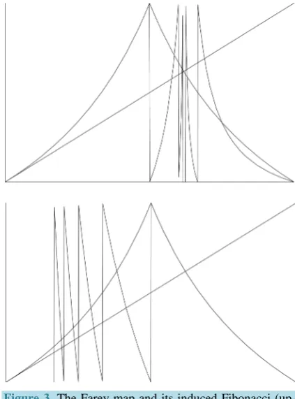
H x = a − a₊  r= i a > (3.31) A sketch of the map F along its induced versions G and H is given in Figure 3.

Given M a b

c d

 

=  

  we may define the Möbius transformation

( )

ˆ _: ax b

x M x

cx d

+

→ =

+

By the above, given x∈

[

0,1 2

]

the point φ−1L−1φ

( )

x is but F x

( )

and for x∈

[

0,1 2

]

we have

( )

1 1

( )

_ˆ1

( )

F x =φ− L− φ x =L− x (recall that 1 1 0

1 1

L− =  _

−

 ). But what happens if x∈

(

1 2 ,1

]

so that

1 1

a = ?

To see this we put

0 1

1 0 0 1

and .

1 1 1 1

I ≡ =L _ _ I =SR=LS=_ _

    (3.32)

We have

3 3

1 2 1 2

1 1

n n

n n n n

I R L R =I L R L 

Therefore, noting that 1 1

1 1 1 0

I− = − _

 , for x∈

(

1 2 ,1

]

we have

( )

( )

( )

1 1 1

1 ˆ1

F x =φ− I− φ x =I− x . To summarize we can represent the action of F as

( )

( )

[

]

( )

(

]

1 0

1 1

ˆ _{, if 0,1 2 ,}

ˆ _{, if 1 2 ,1 ,}

I x x

F x

I x x

−

−

 ∈

 = 

[image:15.595.205.417.83.369.2]

1081

Figure 3. The Farey map and its induced Fibonacci

(up-per) and Gauss (lower) maps.

that of G as

( )

1 ( 1)

_{( )}

1 0

ˆ ˆ n _{, .}

n

G x =I− I− − x x∈A

and that of H as

( )

1 ( 1)

_{( )}

0 1

ˆ ˆ n _{, .}

n

H x =I− I− − x x∈B

3.3.2. The Modified Farey Map

Finally we introduce the modified Farey map F: 0,1

[ ] [ ]

→ 0,1 given by

( )

1

, if 0 ,

1 2

1 1

2 , if 1.

2

x

x x

F x

x x

 _{≤ ≤}

 − = 

 − < ≤ 

 (3.33)

This map preserves orientation and has two indifferent fixed points, at 0 and 1. The advantage of using F

instead of F is that one can retrace the path from a leaf x∈ back to the root 1 2. More precisely, for

x∈ let (cf. Proposition 3.8) _i

i

X =L

∏

M be the element which uniquely represents x in . Then one easily sees that the following rule is in force: if F( )i−1

( )

x <1 2 then M_i =L, F( )i−1

( )

x >1 2 then M_i =R, for i=1,,k with k=rank

( )

x so that Fk

( )

x =1 2.

4. The Minkowski Question Mark

Given a number

x

∈

( )

0,1

with continued fraction expansion x=

[

a a a₁, ₂, ₃,

]

, one may ask what is the number obtained by interpreting the sequence

φ

( )

x

(see (3.14)) as the binary expansion of a real number in

(0,1). The number so obtained is denoted

?

( )

x

and writes

( )

2

1 1 3

? 0.00 011 100 0

a

a a

x

−

or, which is the same,

( )

( )

1 (1 1)

1

?

1

k

2

a ak

.

k

x

− − + + −

≥

=

∑

−



(4.2) For instance ? 1

( )

n =1 2n−1, for all n≥1 (see Figure 4). Setting ? 0

( )

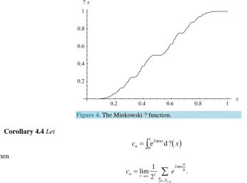
=0 and ? 1

( )

=1 one has the following properties for the function ? : 0,1

[ ] [ ]

→ 0,1 (see [13]-[16]):

• ?

( )

x is strictly increasing from 0 to 1 and Hölder continuous of exponent

(

log 2

)

2 log 5 1 2

β =

+ ;

• x is rational iff ?

( )

x is of the form

_k

2

s _{, with k and s integers;}

• x is a quadratic irrational iff ?

( )

x is a (non-dyadic) rational;

• ?

( )

x is a singular function: its derivative vanishes Lebesgue-almost everywhere. The following additional properties easily follow from the definition.

Lemma 4.1 ?

( )

x satisfies the functional equations

(

) ( ) ( )

? 1−x =? 1 −? x

( )

1

? ? , 0 1 2

2 1

x

x x

x

 

= _{ } ≤ ≤

−

 

Proof. Assuming that x∈

[

1 2 ,1

]

we write

x

=

1

(

y

+

1

)

with y∈

[ ]

0,1 and 1− =x y

(

y+ ∈1

)

[

0,1 2

]

. Setting moreover y=

[

a a₁, ₂,

]

we have x=

[

1,a a₁, ₂,

]

and 1− = +x

[

1 a a₁, ₂,

]

. The assertion now follows by direct application of (4.2). ♦

Let us now see how ? acts on Farey fractions. We have already seen that

( ) ( )

1 0 1 1 1

? ? ? 0 ? 1

2 1 1 2 2

+

 ₌  _{=  + =}

   ₊   

   

More generally, for any pair a b and a b′ ′ of consecutive Farey fractions the function ? equates their child to the arithmetic average:

1

? ? ?

2

a a a a

b b b b

′ ′

+  

 ₌  ₊    _{+ ′}     _′ 

       (4.3) One sees that the function ? maps the Farey tree  to the dyadic tree



defined as follows: having fixed

1 ≥

 , let _ be the ascending sequence of fractions of the form _{k 2}−1_, 1 0,1, , 2

k=  − . We have

1 2 3

0 1 0 1 1 0 1 1 3 1

, , , , , , , , ,

1 1 1 2 1 1 4 2 4 1

     

=_{ } =_{ } =_{ }

     

  

and so on. Then



is the same graph as  with the



-th row replaced by   _{+1 }. An immediate con- sequence of the fact that ?

( )

 = is that ?

( )

x is the asymptotic distribution function of the sequence of Farey fractions:

Theorem 4.2 Since

1

# :

lim

2

a a

x

b b

x

+

→∞

 _{∈ ≤} 

 

 

= _





then

( )

# 1:

? lim

2

a a

x

b b

x

+

→∞

 _{∈ ≤} 

 

 

= _ ⋅





Remark 4.3 This result can be also deduced as a consequence of a more general result obtained in [17] using a suitable enumeration of the rationals in

( )

0,1 . As for the convergence of the atomic measure concentrated on

n

 to d? see [11] and [18].

[image:16.595.253.375.564.658.2]

[image:17.595.91.440.87.344.2]

1083

Figure 4. The Minkowski ? function.

Corollary 4.4 Let

( )

1 2π 0e d ?

inx n

c =

∫

x

then

1

2π 1

lim .

2

a in

b n

a b

c e

+ →∞

∈

=

∑



 



Finally, a short reflection using the definition (4.1) shows that ? conjugates the Farey map F and the modified Farey map F to the tent map

( )

2 ,

₍

₎

if 0 1 2 ,

2 1 , if 1 2 1.

x x

T x

x x

≤ < 

=  _{− ≤ ≤}

 (4.4)

and the doubling map

D x

( )

=

2 mod1

x

, respectively. Indeed, for any ω ω ω= _{1 2} with

ω ∈

_i

{ }

0,1

we have

0.00 01 0.00 01 for

i

k k i

T

ω

ω

i k

−

 _{ = ≤}

 

    (4.5)

and

(

0.1

)

0.

T

ω

=

ω

(4.6) where ω ω ω= _{1 2} and ωi= −1 ωi. A similar reasoning applies for D. Putting together the above, (3.25) and

(4.1) we then get the following commutative diagrams

Theorem 4.5

[ ]

[ ]

[ ]

[ ]

[ ]

[ ]

[ ]

[ ]

0,1 0,1 0,1 0,1

? ? , ? ?

0,1 0,1 0,1 0,1

F F

T D

→ →

↓ ↓ ↓ ↓

→ →



This implies that the measure

d

?

( )

x

is invariant under both maps F and F, and its entropy is equal to

log 2. This makes

d

?

( )

x

the measure of maximal entropy for F and F. Being zero at every rational point ?

d is of course singular w.r.t. Lebesgue. More specifically, d? is concentrated on a subset X ⊂

[ ]

0,1 having Hausdorff dimension α≈0.875 (see [14]). In view of (3.25), the above has the following straightforward consequence

Lemma 4.6 If x is drawn from

[ ]

0,1 according to the singular measure

d

?

( )

x

, then the partial quotients

( )

a

_{i i≥1} of x=

[

a a₁, ₂,

]

form a sequence of i.i.r.v.’s with Prob

(

)

2 n i

a =n = − .

It is moreover easy to realize that F and F have also absolutely continuous (not normalizable) invariant measures, with densities 1x and 1x

(

1−x

)

, respectively.

5. Transfer Operators and Partition Functions

To a given matrix M a b

c d

 

=_{ }∈

   and complex parameter q one can associate the positive operator

( )

q M

π acting on the right as [20]

( ) ( ) (

)

2 _ˆ

( )

(

_ˆ

( )

)

: q q .

q

ax b

M f x cx d f M x f M x

cx d

π

_{= +} −  + _{= ′ ⋅}

 ₊ 

  (5.1)

For example we have

( ) ( )

2

1 1

.

q S f x q f

x x

π

=  _{ }

  (5.2)

The operator _q associated in this way to the map

(

[ ]

0,1 ,F

)

turns out to be the transfer operator acting as

( )

( )

( ) ( )

(

)

0 1 2

1 1

: .

1 1

1

q q q q

x

f x I I f x f f

x x

x

π π     

 

=_ + _ = _{  }+ _{ }

+ +

   

+  

 (5.3)

Of special significance is the (Perron-Frobenius) operator ₁ which satisfies

( ) ( )

( )

( )

1 1

1

0g F x f x dx= 0g x f x dx

∫



∫

 (5.4)

and has norm at most one in the Banach space L1

(

[ ]

0,1 , dx

)

. A function h is the density of an absolutely continuous invariant measure for F if and only if ₁h=h. In this case we find h x

( )

=1x, which however does not lie in L1

(

[ ]

0,1 , dx

)

(see [21]).

Let f be an eigenfunction of _q analytic in the half-plane Rex>0. It satisfies

( )

( )

1 2 1

1 1 1

q

q

x

f x f x f f

x x x

λ = =_{ } _ _ _+ _ __

+ + +

      

 (5.5)

and also

( ) ( )

( )

q S f x f x

π

= (5.6) Therefore the eigenvalue equation is equivalent to the three-term equation

( )

(

)

2

1 1

1 _q 1

f x f x f

x x

λ

= + + _ + _

  (5.7)

which is a generalisation of the Lewis functional equation (with λ=1) studied in number theory (see [20] [22]). The study of this generalized equation has been initiated in [23].

Remark 5.1 In the context of the thermodynamic formalism, once a one-sided shift Φ Σ → Σ: and a potential function

ϕ

∈C

( )

Σ are given one defines a transfer operator ϕ on C

( )

Σ by

( )

( )

_{( )}

1 e

g ϕ η g

ϕ

η ξ

ξ η

− ∈Φ =

∑



which plays a key role in the study of equilibrium states for

(

Σ Φ

, ,

ϕ

)

and their properties [24] [25]. In parti- cular, one defines

( )

( )

{

}

var_kϕ=sup ϕ ξ −ϕ ξ′ :ξ_i=ξ_i′, 0< ≤i k

and it turns out that if varkϕ decays exponentially then there is a unique mixing equilibrium state.

Relying on the above discussion it is now easy to see that

φ

_*_q=_ϕ with

( )

(

1

( )

)

2 log 1q .

ϕ ξ

_{= − +}

φ ξ

−

In order to compute varkϕ we have to consider points sharing the same path up to the k-th row of . Take

for instance

ξ

=

L

∞ and ξ′ =_{L R}k _{. Then a short reflection yields, for} 0

q≠ ,

( )

( )

C