IRIS Classification based on Fractal Dimension Box Counting Method

IRIS Classification based on Fractal Dimension Box

Counting Method

Pravin S.Patil

Electronics and Communication Engineering Department,

SSVPS`s B.S. Deore College of Engineering Dhule.

ABSTRACT

Among many biometrics approaches, iris recognition is known for its high reliability, but as databases grow ever larger, an approach is needed that can reduce matching time. This can be easily achieved by using iris classification This paper presents fractal dimension box counting method for classifying the iris images into four categories according to texture pattern. Initially eye image is localized by using random circular contour method than a preprocessed flat bed iris image of 256 64 size is generated, which is further divided into sixteen regions. Eight regions are drawn from the middle part of the iris image, The remaining eight regions are drawn from the bottom part of the iris image. From these sixteen regions sixteen 32×32 image blocks are generated. To calculate the fractal dimensions of these image blocks box counting method is used. This produces sixteen fractal dimensions. The mean values of the fractal dimensions of the two groups are taken as the upper and lower group fractal dimensions; respectively The double threshold algorithm uses to classify the iris into the four categories.Peformance of the implemented algorithms have been evaluated using confusion matrix and experimental results are reported. The classification method has been tested and evaluated on CASIA V1 iris database.

General Terms

Security,Biometrics Iris Recognition

Keywords

Iris Classification,Fractal Dimensions,Double Threshold Algorithm

1. INTRODUCTION

The iris classification and indexing can be used to filter the search space during identification process and are still considered as interesting but difficult problem in image processing.[1][2] Suppose there are a finite number of iris classes

𝐶

_𝑖,

𝑖 = 1, 2,3, … . , 𝑛

and a number of training samples of each class are available. Based on the information extracted from the training samples, a decision rule is designated which classifies a given sample of unknown class into one of the

𝑛

classes. To design an effective algorithm for iris classification, it is essential to find a set of iris textural features with good discriminating power.[3][4] Very few techniques for classifying iris images have been proposed in the literature that characterizes the features based on frequency contents and orientation of different iris textures. These methods characterize the spatial frequency contents, but do not consider the information in the spatial domain.[5] Information regarding the spatial frequency alone is not adequate enough in many cases, especially when the iris

textures are non-stationary. The non-stationary behavior of the iris textures is due to local variation in size, orientation and frequency of the texture elements.[6] For analyzing such textures of irises, one has to take into consideration the spatial as well as spatial frequency characteristics of the iris image. In such cases, feature extraction method should yield a spatial/spatial-frequency representation that is orientation-sensitive.[7][8] These methods overcome lack of locality in the frequency analysis methods. The fractal dimension has been used in image classification to measure surface roughness where different natural scenes such as mountains, clouds, trees, and deserts generate different fractal dimensions.[9][10][11] The box counting method is widely used for classification, as it can be computed automatically and can be applied to patterns with or without self-similarity. The input iris image have been classified by using a fifteen step algorithm as below:

Step 1: Read original eye image from CASIA V1 database Step 2: Marked random circular contour and formation of circular pseudo image.

Step 3: This circular pseudo image is then convolved with the eye image from the database.

Step 4: Formation of Binary Pupil Image

Step 5: Alignment of iris in the center of the frame Step 6: Formation of Semi-circular limbus after gray level

slicing.

Step 7: Localized iris by marking pupillary and sceleric

boundaries. Step 8: Iris after removal of the eyelids.

Step 9: Extraction of flat bed iris for the region closer to the pupil

Step 10:Formation of Estimated background illumination iris image

Step 11: Enhanced unwrapped iris image of 256 × 64 image block..

Step 12: Separate the iris image into sixteen image blocks measuring 32 × 32 pixels.

Step 13: Calculate the fractal dimension using the box-counting method and obtain two mean fractal dimensions

values. Step 14: Using double threshold algorithm classify the iris

images into one of the defined categories.

2. IRIS LOCALIZATION

2.1 Circular Iris localization using Random

Circular Contour Method

In this method, initially any random circular contour is marked which contains iris and pupil region to eliminate the remaining portion of the eye. A circular pseudo image is formed of the desired diameter. The inside region of the circle is set at gray level „1‟(white) and the outside region to „0‟(black).[12] The diameter selected empirically in such way that the circular contour will encircle the entire iris. This diameter selection is crucial as it should be common for all iris images.This circular pseudo image is then convolved with the eye image from the database.[12] Thus when the product of the gray levels of the circular pseudo image and the original iris image has been taken, the resultant image will have the circular contour enclosing the iris patterns and the outside of the circular contour will be at gray level „0‟(black). The results for marking random circular contour have been illustrated in Figure 1.

(a)

[image:2.595.315.551.97.253.2]

(b)

Figure 1. Formation of random circular contour around the iris (a) original eye in CASIA database (01_1_2.bmp),

(b) marked random circular contour.

The resultant image Figure 1. (b) is the partial localized iris image. And the other task is to move this circular contour in such a way that it is concentric with the pupil. This alignment is required since minor shifts often occur due to offsets in the position of the eye along the camera‟s optical axis. So before pattern-matching, alignment is carried out. The limbus and pupilary boundary of the iris are concentric about the pupilary center.

To determine the pupilary centere we used point image processing techniques such as thresholding and gray-level slicing (without the background) on the resultant partially localized image to eliminate the other features of eye except the pupil of the eye. The pupil of the eye is set at gray level

[image:2.595.58.278.282.568.2]

„0‟ (black) and rest of the region is set at „255‟ (white). The resultant pupil image has been illustrated in Figure 2.

Figure 2. Pupil Image of the random circular contour around the iris .

Then the resultant pupil image is scanned row-wise to determine the number of pixels having gray level „0‟ in each row and the maximum count have been considered as the diameter of the pupil along the row. Now scanning the resultant pupil image column-wise, a counter will count the number of pixels having gray level „0‟ in each column and the maximum count has been considered as the diameter of the pupil along the column. Taking the average of the two, we have obtained the average of the pupil diameter.

Next step involves determining the center of the pupil. This is done by finding the row and column having the maximum number of pixels of gray level „0‟ (black), which corresponds to the center of the pupil. Knowing the center of the pupil, we now shift the center of the circular contour to the center of the pupil. The resultant image will have the pupil and the iris regions concentric with the circular contour. The image obtained from the circular contour encircling the pupil and the iris is not at the center of the frame. So the step in the alignment involves shifting the circular contour to the center of the frame. Knowing the center of the frame and the center of the circular contour, the difference in the two centers can be determined.

Using this difference, gray level shifting on the image has been carried out appropriately. The resultant image will have the center of the circular contour coinciding with the center of the frame. This has been illustrated in Figure 3.

[image:2.595.323.536.571.716.2]

[image:3.595.323.536.129.318.2]

In order to determine the limbus diameter we have used image point processing operators, mainly gray level slicing with and without the background and a digital negative, we obtain only the iris at gray level „0‟ (black) and the remaining portion of the image is at gray level „255‟ (white) . The shape of the limbus in this case can be considered to be semi-circular as shown in Figure 4.

Figure 4. Semi-circular limbus after gray level slicing.

Now scanning row-wise, a counter determines the number of pixels having gray level „0‟ (black) in each row and the maximum count can be considered as the diameter of the limbus along the row. Now scanning column-wise, a counter determines the number of pixels having gray level „0‟ (black) in each column and the maximum count can be considered as the radius of the limbus. Doubling gives the diameter of the limbus along the column. Taking the average of the two, we get the average limbus diameter. Then, the ratio of the limbus diameter and the pupil diameter is determined which is the basis of the first criterion in identification / comparison of the iris.

Finally, the result of iris localization of the eye with iris (limbus) and pupil are circled correctly in the aligned iris image has been demonstrated in Figure 5.

Figure 5. Aligned Iris in eye marked with circles for iris and pupil boundaries.

[image:3.595.61.273.149.344.2]

The eyelids/eyelashes are occluding part of the iris, so only the portion of the image below the upper eyelids and above the lower eyelids are included.[14] Thus removing the portion of the iris occluded by the eyelids/eyelashes is the next task to perform. Figure 6.

Figure 6. Resultant iris after removal of the eyelids / eyelashes.

2.2 Flat Bed Iris Localization

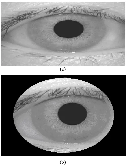
The homogenous rubber sheet model takes into account pupil dilation and size inconsistencies in order to produce a normalized representation with constant dimensions. In this way the iris region is modeled as a flexible rubber sheet anchored at the iris boundary with the pupil centre as the reference point. Even though the homogenous rubber sheet model accounts for pupil dilation, imaging distance and non-concentric pupil displacement, it does not compensate for rotational inconsistencies.[15]

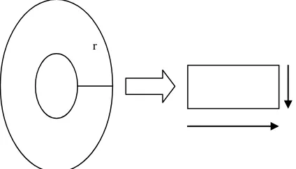
The dimensional inconsistencies between eye images are mainly due to the stretching of the iris caused by pupil dilation from varying levels of illumination. Other sources of inconsistency include, varying imaging distance, rotation of the camera, head tilt, and rotation of the eye within the eye socket.[16] Another point of note is that the pupil region is not always concentric within the iris region, and is usually slightly nasal. This must be taken into account if trying to normalize the „donut‟ shaped iris region to have constant radius. We can remap each point within the iris region to a pair of polar coordinates (r, θ) where r is on the interval [0, 1] and θ is the angle between [0, 2π]. Figure 7. shows simple implementation of the iris unwrapping.

r

r r

θ

[image:3.595.61.276.533.708.2] [image:3.595.319.531.618.739.2]

The remapping of the iris region from (x, y) Cartesian coordinates to the normalized non-concentric polar representation is modeled as,

𝐼(𝑥 𝑟, 𝜃 , 𝑦 𝑟, 𝜃 ) → 𝐼(𝑟, 𝜃)

(3.5) with

𝑥 𝑟, 𝜃 = 1 − 𝑟 𝑥

_𝑝

𝜃 + 𝑟 𝑥

₁

𝜃

(3.6)

𝑦 𝑟, 𝜃 = 1 − 𝑟 𝑦

_𝑝

𝜃 + 𝑟 𝑦

₁

𝜃

(3.7)

where,

I(x, y) is the iris region image,

(x, y) are the original Cartesian coordinates, (r, θ) are the corresponding normalized polar coordinates,

𝑥

_𝑝,

𝑦

_𝑝 are the coordinates of the pupil, and

[image:4.595.55.285.383.525.2]

𝑥

₁,

𝑦

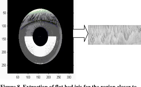
₁ are the iris boundaries along the θ direction. The iris region closer to the pupil and scelera contributes the least to the discriminating information contained within the iris.[17] Also this region rarely occluded by eyelids and eyelashes.[18] So we extract the flat bed iris for the region closer to the pupil as illustrated in Figure 8.

Figure 8. Extraction of flat bed iris for the region closer to the pupil.

[image:4.595.53.269.668.718.2]

The unwrapped normalized iris image still has low contrast and may have non-uniform brightness caused by the position of light sources. All these may affect the subsequent feature extraction and matching.[16] In order to obtain a better distributed texture in the iris, we first approximate intensity variations across the whole iris image. The mean of each small block (we have considered the size of each block as 16×16 empirically) constitutes a coarse estimate of the background illumination.[16] This estimate is further expanded to the same size as that of the normalized image by using bi-cubic interpolation. Figure 9.

Figure 9. Estimated background illumination.

This estimated background illumination is subtracted from the unwrapped normalized image to compensate for a variety of lighting conditions.[16] Then we enhance the lighting corrected image by means of histogram equalization in each (32×32) region. Such processing compensates for non-uniform illumination, as well as improving the contrast of the image. Figure 10.

Figure 10. Enhanced unwrapped iris image.

3. IRIS CLASSIFICATION USING

FRACTAL DIMENSION BOX

COUNTING METHOD

In the box-counting method, an image measuring size R×R pixels is scaled down to s×s, where

1 < 𝑠 ≤ 𝑅 2

, and s is an integer. Then

𝑟 = 𝑠 𝑅

. The image is treated as a three-dimensional space, where two dimensions define the coordinates (x, y) of the pixels and the third coordinate (z) defines their grayscale values. The (x, y) is partitioned into grids measuring s×s. On each grid there is a column of boxes measuring s×s×s. If the minimum and the maximum grayscale levels in the (i, j)th _{grid fall into, the k}th _{and l}th _boxes respectively, the contribution of

𝑛

_𝑟 in the (i, j)th grid is defined as,

𝑛

_𝑟

𝑖, 𝑗 = 𝑙 − 𝑘 + 1

(1)

In this method Nr is defined as the summation of the

contributions from all the grids that are located in a window of the image,

𝑁

_𝑟

= 𝑛

_{𝑖,𝑗 𝑟}

𝑖, 𝑗

(2) If

𝑁

_𝑟 is computed for different values of r, then the fractal

dimension can be estimated as the slope of the line that best fits the points

(log 1 𝑟

, log 𝑁

_𝑟

)

. The complete series of steps for calculating the fractal dimension are as follows. First, the image is divided into regular meshes with a mesh size of r. We then count the number of square boxes that intersect with the image

𝑁

_𝑟. The number

𝑁

_𝑟 is dependent on the choice of r. We next select several size values and count the corresponding number

𝑁

_𝑟. Then the final equation used to estimate the fractal dimension is,

log 𝑁

_𝑟

_{= log 𝐾 + 𝐷 log(1 𝑟}

)

(3) where,

K is a constant and

D denotes the dimensions of the fractal set.

The whole basic theory explained above is applied on normalized image i.e. slab which can be observed from normalization process explained earlier.

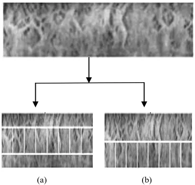
In our experiments, the preprocessed images were transformed into images measuring 256 64. Because all iris images have a similar texture near the pupil, we do not use the upper part of the iris image when classifying an iris.

iris image. Preliminarily, we use the box-counting method to calculate the fractal dimension.[19] To do this, we first divide a preprocessed iris image into sixteen regions. Eight regions are then drawn from the middle part of the iris image, as shown in Figure 11.

[image:5.595.68.267.128.317.2]

(a) (b) Figure 11. Image segmentation: (a) upper group and (b)

lower group.

We call these the upper group. The remaining eight regions are drawn from the bottom part of the iris image. These are referred to as the lower group. From these sixteen regions we obtain sixteen 32×32 image blocks. We then use the box-counting method to calculate the fractal dimensions of these image blocks.[20] This produces sixteen fractal dimensions,

𝐹𝐷

_𝑖

(𝑖 = 1, 2, … ,16)

. The mean values of the fractal dimensions of the two groups are taken as the upper and lower group fractal dimensions, respectively

𝐹𝐷

_{𝑢𝑝𝑝𝑒𝑟}

=

8𝑖=1𝐹𝐷𝑖

8 (4)

𝐹𝐷

_{𝑙𝑜𝑤𝑒𝑟}

=

16𝑖=9𝐹𝐷𝑖

8 (5)

Classification of an iris using the double threshold algorithm: Once we have determined the values of the upper and the lower group fractal dimensions, we can classify the iris image using the double threshold algorithm.[19] The double threshold algorithm uses two thresholds to classify the iris into the following four categories, according to the values of the upper and lower group fractal dimensions. The categories have been decided on the basis of;

Category 1 : The values of both the upper and lower group fractal dimensions are less than the first threshold.

𝐹𝐷

𝑢𝑝𝑝𝑒𝑟

, 𝐹𝐷

𝑙𝑜𝑤𝑒𝑟

𝐹𝐷

𝑢𝑝𝑝𝑒𝑟

<

𝐸

₁

𝐴𝑁𝐷 𝐹𝐷

_{𝑙𝑜𝑤𝑒𝑟}

< 𝐸

₁ (6)

Category 2: The values of the upper group fractal dimensions is greater then E2 and lower group fractal dimensions are grater then the E2.

𝐹𝐷

𝑢𝑝𝑝𝑒𝑟

, 𝐹𝐷

𝑙𝑜𝑤𝑒𝑟

𝐹𝐷

𝑢𝑝𝑝𝑒𝑟

>

𝐸

2

𝐴𝑁𝐷 𝐹𝐷

𝑙𝑜𝑤𝑒𝑟

> 𝐸

2 (7)

Category 3: The values of the upper group fractal dimensions is less then E2 and lower group fractal dimensions are grater then the E2.

𝐹𝐷

_{𝑢𝑝𝑝𝑒𝑟}

, 𝐹𝐷

_{𝑙𝑜𝑤𝑒𝑟}

𝐹𝐷

_{𝑢𝑝𝑝𝑒𝑟}

<

𝐸

2

𝐴𝑁𝐷 𝐹𝐷

𝑙𝑜𝑤𝑒𝑟

> 𝐸

2 (8)

Category 4: When the upper and lower group fractal dimension values of an iris fail to satisfy the rules of categories 1, 2, or 3, they are classified into category 4.

4. RESULTS AND DISCUSSIONS

The proposed algorithms have been developed using MATLAB 7.1. It is tested on 2.4 GHz CPU with 2 GB RAM. The famous iris database CASIA-Iris, which is currently the largest iris database available in the public domain have been selected for experiments.[21]

Table 1. Iris database (CASIA V1).

S SESSION-1 SESSION-2

1

01_1_1.bmp 01_2_1.bmp

2

01_1_2.bmp 01_2_2.bmp

3

[image:5.595.298.558.303.754.2]

4

[image:6.595.49.288.208.766.2]

01_2_4.bmp

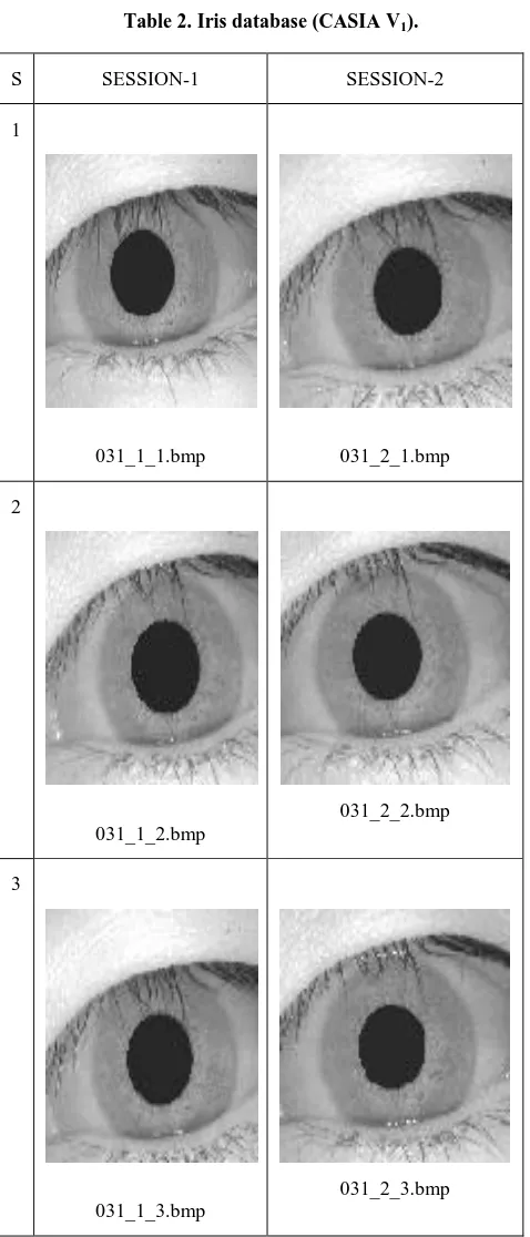
Table 2. Iris database (CASIA V1).

S SESSION-1 SESSION-2

1

031_1_1.bmp 031_2_1.bmp

2

031_1_2.bmp

031_2_2.bmp

3

031_1_3.bmp

031_2_3.bmp

4

031_2_4.bmp During experimentations the threshold values E1 and E2 for comparisons with the

𝐹𝐷

_{𝑢𝑝𝑝𝑒𝑟} and

𝐹𝐷

_{𝑙𝑜𝑤𝑒𝑟} have been decided empirically as,

First threshold, E1=2.9194 Second threshold, E2=2.7578

[image:6.595.308.549.483.600.2]

To evaluate the feasibility and performance of the algorithm for the iris recognition task, the eye images from the CASIA V1 iris database are used, which is a standard test bed for iris recognition technologies. Extensive experiments on image database have been performed to evaluate the effectiveness and accuracy of the work. From the database we have selected 372 iris images From 108 different eyes (under different conditions) of 54 subjects. The images are acquired during different stages and the time interval between two collections is at least one month, which provides a challenge to the algorithm. The profile of the database for two different eye images is shown in Table 1. and Table 2. The fractal dimension values of the four categories of iris have been illustrated in Table 3.

Table 3. Fractal dimension values of the four categories of iris.

FD Category 1

Category 2

Category 3

Category 4

𝐹𝐷𝑢𝑝𝑝𝑒𝑟 2.8319 2.6286 2.9190 2.8149

𝐹𝐷𝑙𝑜𝑤𝑒𝑟 2.8218 2.5110 2.6222 2.7571

5. PERFORMANCE EVALUATION OF

CLASSIFICATION ALGORITHMS

[image:7.595.43.292.84.255.2]

Table 4. Confusion matrix for CASIA V1 test set.

True Class Assigned Class

Category 1

Category 2

Category 3

Category 4

Category 1 94% 0 0 6%

Category 2 0 96% 4% 0

Category 3 0 5% 87% 8%

Category 4 0 3% 6% 91%

6. CONCLUSION

This paper presents an iris classification algorithm based on the box-counting method of fractal dimension. Accurate and consistent Iris classification provides an important indexing mechanism for personal identification. Also it can greatly reduce iris-matching time and computational complexity for a large database as the input iris needs to be matched only with a subset of the iris database.. The average accuracy obtained for classifying all the images was observed to be 92%.

7. REFERENCES

[1] J. Daugman (1994), “Biometric Personal identification System based on iris analysis”, US patent no. 529160. [2] J. Daugman,(2007), “New methods in Iris Recognition,”

IEEE transactions on systems, man and cybernetics-part B:Cybernetics 37(5), 1167-1175

[3] Z.Sun (2014), “Iris Image classification Based on Hierachical Visual Codebook” ,” IEEE Transactions on pattern analysis and machine intelligence.36 (.6), 1120-1133.

[4] E. Srinivasa Reddy and I. Ramesh Babu,(2007) “Biometric template classification: A case study in iris textures,” ICGST-BIME Journal, vol.7, issues 1, pp 17-22

[5] J. Daugman (2003), “Demodulation by Complex valued wavelets for stochastic pattern recognition”, International Journal of Wavelets, Multiresolution and Information Processing, 1(1), 1-17

[6] P.Perona (1998) “ Orientation Diffusion”,IEEE Transction on Image Processing,vol.7,pp.457-467 [7] M. Tuceryan and A. Jain. Texture analysis. In C. H.

Chen, L. F. Pau, and P. S. P. Wang,(1993) “Handbook Pattern Recognition and Computer Vision” World Scientific Publishing,pp 235-276

[8] Z.Sun,Y.Wang,T.Tan,J.Cui (2004) “ Robust Direction Estimation of Gradient Vector Field for Iris Recognition” IEEE International Conference

[9] A.P. Pentland (1984) “ Fractal-based description of natural scenes,” IEEE Transactions on Pattern Analysis

and Machine Intelligence 6 pp 661–674. [10]B.B. Mandelbrot (1982) “The Fractal Geometry of

Nature, Freeman, San Francisco,” CA, [11]B.B. Chaudhuri, N Sarker (1995) “ Texture segmentation

using fractal dimension,” IEEE Transactions on Pattern Analysis and Machine Intelligence 17, 72–77

[12]Pravin S.Patil (2012) “Iris Recognition Based on Gaussian-Hermite Moments” International Journal Computer Science and Engineering.(IJCSE),.4(11) 1794-1803

[13]Pravin S.Patil, Satish R.Kolhe (2010) “Robust Porsonal Identification using Iris” Ascent Journals, International Journal for Engineering Research and Industial Application.(IJERIA) 3(4) 165-177

[14]W. Kong, D. Zhang (2001) “Accurate iris segmentation based on novel reflection and eyelashes detection model,” Proceeding of International symposium on intelligent multimedia, video and speech processing Hong Kong

[15]J. Daugman (2006) Probing the uniqueness and randomness of iriscodes: Results from 200 billion iris pair comparisons. Proceedings of the IEEE, 94(11) [16]L.Ma, T. Tan (2003) Y.Wang, and D. Zhang “Personal

identification based on iris texture analysis,” IEEE Transactions on Pattern Analysis and Machine Intelligence, 25(12), 1519–1533

[17]J. E. Gentile, N. Ratha, and J. Connell.(2009) SLIC : Short-length iris codes. IEEE 3rd International Conference on Biometrics: Theory, Applications, and Systems (BTAS),

[18]H. Sung, J. Lim, Y. Lee (2004) “Iris recognition using collarette boundary localization,” Proceeding of the 17th International conference on pattern recognition

[19]LiYu,,D. Zhang, K.Wang,W.Yang (2005) “ Coarse iris classification using box-counting to estimate fractal dimensions” Elsevier Journal of Pattern Recognition, 38 1791 – 1798

[20]LiYu,, K.Wang, D. Zhang (2005) “ Coarse iris classification using box-counting method” IEEE Conference on Image Processing(ICIP), .3 301-304

[21] “CASIA Iris Image Database,”

http://www.sinobiometrics.com