Vector Control of Induction Motor Using ANN and Particle Swarm Optimization

(1)

International Journal of Emerging Technology and Advanced Engineering

Website: www.ijetae.com (ISSN 2250-2459, Volume 2, Issue 9, September 2012)

480

Vector Control of Induction Motor Using ANN and

Particle Swarm Optimization

Aeidapu Mahesh

1

_{, Dr. Balwinder Singh}

2

1_{PG student, Department of Electrical Engineering, PEC University of Technology, Chandigarh, India}

2_{Department of Electrical Engineering, PEC University of Technology, Chandigarh, India}

Abstract--- This paper presents the scheme of vector control of Induction Motor using three different types of speed controllers, conventional PI controller, ANN speed controller and PI controller, for which parameters are optimized using Particle Swarm Optimization technique. The disadvantage of the PI controller like slow response and large settling time are avoided using the ANN speed controller. The data used to train the ANN controller is taken from the simulation of conventional controller. As the third method particle swarm optimization technique was used to optimize the parameters of PI controller by considering the maximum peak overshoot as the error function. The advantage of the optimized controller is there is no need to change in the design part of the vector control scheme. The simulation results indicate the optimized controller possesses excellent dynamic response at all reference speeds. The results for conventional controller, ANN controller and optimized controller are shown at the end.

Key words--- Vector Control, PI controller, Particle Swarm Optimization (PSO)

I. INTRODUCTION

The vector control or also known as Field Oriented Control has been widely used in the induction motor control has been established as the core servo-drive system for industry application [1]. The vector control uses the dynamic mathematical model of induction motor and decouples control of flux and torque which makes the induction motor deliver excellent dynamic performance [2]. In order to get good dynamic performance the parameters of the speed controller must be accurate. The methods given in reference [3-5] using ANN and Fuzzy logic are rendering good performance but they require the additional components in the design, thus increasing the cost of the system.

The proposed system uses only the regular PI speed controller, but the parameters are optimized using Particle Swarm Optimization. This method uses the maximum peak as the fitness function and the Proportional gain (Kp) and

the Integral Gain (Ki) as the control parameters.

MATLAB/Simulink is used to perform the Simulation and the programming part. The detailed explanation and the discussion are presented in this paper.

II. MATHEMATICAL MODEL OF INDUCTION MOTOR

The dynamic model of the induction motor is developed by converting the three phase quantities into two phase quantities. The quantities are converted to two phase because of the conceptual simplicity obtained with the two windings. The power invariance is used to observe the equivalence between three phase and two phase machine models. The transformations are used to transform the motor parameters like voltage, currents and the flux linkages from three phase to the two phase rotating or stationary rotating reference frames.

The mathematical model of a squirrel cage Induction motor in rotating reference frame [6] is given by:

(2)

International Journal of Emerging Technology and Advanced Engineering

481

Where, Rs and Rr are the stator and rotor resistances, Ls and

Lm are the stator and rotor self-inductances respectively, Lm

is the mutual inductance, ωs is the rotary angular velocity

of the d-q frame of axes,ωslis the slip angular velocity, p is

the derivative operator, λ ,V ,i and are the rotor flux, stator voltage, and stator current respectively.

III. STRATEGY OF INDIRECT VECTOR CONTROL

The simplicity obtained by using separately excited dc drives is that the flux and torque can be independently controlled, and by maintaining the field flux constant, independent control of the torque is possible. Moreover, for controlling of the dc drives, only the magnitudes of the armature and field currents are required, but in case of ac motor speed control we require magnitude along with the phase, which makes the ac motor control difficult

.

By contrast, ac introduction motor drives require a coordinated control of stator current magnitudes, frequencies, and their phases, making it complex control. To make the ac motor control similar to the dc motor control the stator current phasor is resolved, into two parts, one along the rotor flux linkages, and the other in quadrature which is a torque producing component. Once these currents are available then the ac motor can be controlled very much similar to the dc motor [6-7].

The Indirect Vector Control strategy is built based on the mathematical model corresponding to the equivalent model of Induction Motor. The indirect vector control scheme accepts the flux and speed commands and generates the torque producing and flux producing components of the stator current phasor and the slip angle Өsl commands. The command slip angle Өsl* is generated

by integrating ωsl*. The field angle Өf is obtained by the

command slip angle and rotor angle Өr [6].

The equations related to the indirect vector control strategy are given below:

Fig 1. Diagram of typical indirect vector control scheme.

IV. ARTIFICIAL NEURAL NETWORKS

A neural network can be defined as “A massively parallel distributed processor made up of simple processing units, which has a natural propensity for storing experimental knowledge and making it available for use”.[8]

It resembles the brain in two respects; one, knowledge is acquired by the network from its environment through a learning process, two, interneuron connection strengths, known as synaptic weights, are used to store the acquired knowledge.

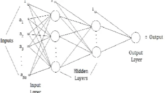
[image:2.612.322.530.115.332.2]

Fig. 2 shows a three layered feed forward neural network. The neural network contains one input layer, one output layer and one hidden layers. The number of hidden layers and the number of the neurons in the hidden layer may be varied depending upon the problem. The neurons which are present in each layer are connected through links. Each and every link is associated with a different connection weight. The inputs to the ith neuron are the outputs from the previous layer of the neurons multiplied by the respective weights.

[image:2.612.360.525.628.721.2]

(3)

International Journal of Emerging Technology and Advanced Engineering

482

The output of each neuron is calculated by using the following equation.

Where, yj is the output of the jth neuron, wij is the

connection weight from jth neuron to ith neuron and n is the

number of previous layer neurons. If the value of the xi

exceeds the activation function value then the neuron gets activated.

The basic concept behind the successful application of neural networks in any field is to determine the weights to achieve the desired target and this process is called learning or training. The two different learning mechanisms usually employed are “supervised” and “unsupervised” learning. In the case of supervised learning the network weights are modified with the prime objective of minimization of the error between a given set of inputs and their corresponding target values [9]. Hence we know the training data set which is a set of inputs and the corresponding targets the neural network should output ideally. This is called supervised learning because both the inputs and the expected target values are known prior to the training of ANN. On the other hand, in the case of unsupervised learning, we are unaware of the relationship between the inputs and the target values. We train the neural network with a training data set in which only the input values are known. Hence it is very important to choose the right set of examples for efficient training.

The structure of the neural network used here is a 2-5-1. It has two inputs namely the reference speed and the actual speed of the motor, has one hidden layer which contains 5 neurons in it and finally it gives one output that is the reference electromagnetic torque. The method used for training the network is supervised learning, the input and target data was taken from the conventional controller.

V. PARTICLE SWARM OPTIMIZATION

Particle Swarm Optimization is a population based stochastic algorithm modeled after the simulation of the social behavior of the bird flocks. Here each swarm or particle has to remember its position and its best position attained so far. The particles are affected by their own experience and also by the other particles in the swarm [8].

The PSO algorithm is an optimizer based on population similar to genetic algorithm. Instead of using the cross over or the mutation as in case of Genetic Algorithm, in PSO the system is initialized with a set of randomly generated solutions called particles, and then it searches for optimal solution iteratively. Each individual particle in PSO flies in the search space with a velocity which is adjusted dynamically according to its own flying experience and also its neighbor‟s flying experience.

The PSO algorithm when compared to Genetic Algorithm has much more profound intelligent background and can be implemented most easily. Due to these advantages the PSO can be used in engineering applications where optimization is required.

Each individual is treated as a particle in a D – dimensional space. And much number of particles forms the population.

Each particle in the PSO is a potential solution, and using an optimization function the particle‟s fitness value is calculated. And the particle with large fitness value is the better particle.

The velocity and the position adjustment are given by (5) and (6) respectively.

In (5), Vid is the speed of particle „i‟ in dimension „D‟.

The first tern in the right hand side corresponds to the inertia force that pushes the particle in its previous direction, where W is called the inertia weight that controls this inertia force. The second term corresponds to the particle‟s individual experience. Here, Xid is the current

location of the particle and Pid is the best position obtained

by the particle so far. C1 is the acceleration coefficient and

rand1 generates the random number between 0 and 1. So,

the second term makes the particle fly towards its individual best from the current position. The third term corresponds to the global best of the particle, and here C2 is

an acceleration constant and rand2 is also a random variable

distributed uniformly in the range of (0, 1). So, this term helps the particle fly in the direction of the global best i.e. the best position found so far among all the particles. For each iteration, according to equation (6), each particle position is adjusted [10].

The parameter W is called inertia weight and it is employed to control the impact of the previous history of velocities on the current one. This parameter is used to regulate the exploration capacity of the swarm. A small value of inertia weight helps in local exploration and a large value in global exploration. So, to reduce the number of iterations required to compute the optimized value, we have to choose a proper value which provides balance between both global and local exploration.

The particle swarm optimization technique doesn‟t use the “survival of the fittest”, like the other optimization techniques, so, each particle in the swarm can be a potential solution.

(4)

International Journal of Emerging Technology and Advanced Engineering

483

This algorithm is defined as:

1. Formulate the initial population and initial velocities randomly.

2. Calculate the fitness function of each particle. 3. Find the individual best of each particle. 4. Find the global best of the entire population. 5. Using equation (5) & (6), update the velocity and

position of each particle.

6. Repeat from step 2 to step 5 until the criterion is satisfied.

VI. SIMULATION AND RESULTS

[image:4.612.326.516.125.341.2]

The proposed vector control system is simulated using MATLAB/Simulink. The induction motor specifications used in the simulation are given below:

TABLE I

PARAMETERS OF INDUCTION MOTOR [1]

Parameters Values

Rated line voltage 460 V Rated speed 183.26 rad/s Pairs of poles 2 Stator resistance (Rs) 0.435 ohm

Stator inductance (Ls) 4 mH

Rotor resistance (Rr) 0.816 ohm

Rotor inductance (Lr) 2 mH

Mutual inductance (Lm) 69.31 mH

During the simulations, at first the parameters of the speed controller Kp and Ki are chosen to be 13 and 26

respectively.

[image:4.612.41.273.327.428.2]

At first the simulation is carried out on no load with a reference speed of 100 rad/sec and then the simulation is repeated with a load torque of 150 Nm applied at 4 sec.

[image:4.612.340.532.483.705.2]

Fig 3. Speed and torque waveforms on no load with 100 rad/s ref speed

Fig 4. Speed and torque waveforms with an applied step load of 150 Nm at 4 sec with 100 rad/s ref speed

From the fig 3 and fig 4, we can see there is some amount of overshoot in the rotor speed every time when there is a change in the system. And the settling time of the motor speed is also high.

The speed controller is now replaced with the ANN speed controller and the same operating conditions as the conventional controller have been performed, and the results are as given below.

[image:4.612.52.240.519.706.2]

(5)

International Journal of Emerging Technology and Advanced Engineering

[image:5.612.65.256.122.323.2]

484

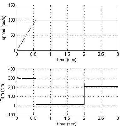
Fig. 6 Rotor speed and electromagnetic torque waveforms with an applied

step load of 200 Nm at T = 2 sec and with a reference speed of 100 rad/s

Fig 5 and fig 6 shows there is no overshoot in speed and the settling time of the speed response is considerably reduced.

As the third method the parameters of the speed controller Kp and Ki are optimized using PSO. The code is

[image:5.612.327.515.124.314.2]

written in MATLAB. The parameters used to perform the PSO are:

Table II: PARAMETERS USED FOR PSO

Parameter Value

Population size 25 Inertia weights Wmin &Wmax 0.4 & 1.0

Acceleration coefficients C1 & C2 1.4 & 2.6

The maximum overshoot in the speed is taken as the error function and the optimization is done online, for every iteration and for every particle the simulation is performed and the final optimized PI parameters obtained as: Kp = 267.7000 and Ki = 0.6863.

[image:5.612.330.519.430.575.2]

Then the simulation is run with the optimized parameters and the results are as shown below:

Fig 7. Speed and torque waveforms on no load with 100 rad/s ref speed

Fig 8. Speed and torque waveforms with an applied load of 150 Nm at 2 sec with 100 rad/s ref speed

[image:5.612.338.532.575.728.2]

Simulation is carried out with the different reference speed commands, at first the speed is chosen to be 80 rad/s, and then increased to 100 rad/s at 2sec then it is increased to 130 rad/s at 2.5sec after that the speed is decreased to 80 rad/s at 3.5 sec.

Fig 9. Rotor speed response in various speed commands

[image:5.612.50.241.588.724.2]

(6)

International Journal of Emerging Technology and Advanced Engineering

[image:6.612.53.241.119.241.2]

485

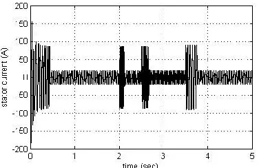
Fig. 11 Stator current waveform in response to various reference speeds

VII.

C

ONCLUSIONS

In this paper various speed controllers for the vector control of the induction motor are successfully demonstrated. As we can see the results obtained from the ANN speed controller and the optimized controller are almost similar. The main advantage of the optimized controller over other speed controllers using ANN or Fuzzy is there is no need for any design changes in the scheme and thereby reducing the cost of the system, so it keeps the advantages of the PI controller such as simple structure and good robustness.

The simulation results show that the new optimized controller gives excellent performance with almost zero maximum peak overshoot. The simulation results also show that the controller possesses very good dynamic response at different reference speed commands. And the controller also has fast response and can be used for real time applications.

REFERENCES

[1]. Wei Jiang, Xiao Yun Feng and Qing Yuan Wang, “Research and simulation on ANN speed-sensorless three-level inverter vector control system for induction motor”, ICEMS 2008, pp 1577 – 1581.

[2]. Chun-shan Lai, Kai-xiang Peng and Gui-shui Cao, “Vector control of induction motor based on online identification and ant colony optimization”, 2nd International Conference on Industrial and Information Systems (IIS), 2010, Vol. 2, pp. 206 – 209.

[3]. Shanmei Cheng, Bo Gong and Jiangcheng Wang, “A novel hybrid speed controller of the vector control system”, ICCAS 2010, pp. 1218 – 1222.

[4]. Miki, I. Nagai, N. Nishiyama, S. Yamada, T. “Vector control of induction motor with fuzzy PI controller” Industry Applications Society Annual Meeting, 1991, Vol. 1, pp. 341 – 346.

[5]. Yang Liyong, Li Yinghong; Chen Yaai and Li Zhengxi, “A novel fuzzy logic controller for indirect vector control induction motor drive”, WCICA 2008, pp. 24 – 28.

[6]. R. Krishnan, “Electric Motor Drives Modeling, Analysis and Control”, PHI learning private Ltd., 2001.

[7]. Bimal K. Bose, Modern Power Electronics and AC Drives, China Machine Press, 2002.

[8]. Simon Haykin, “Neural networks, a comprehensive foundation”, 2nd_{edition, Pearson Prentice hall, 2005.}

[9]. Eberhart, Yuhui Shi, “Particle swarm optimization: developments, applications and resources”, congress on Evolutionary Computation, 2001, Vol. 1,pp. 81 – 86.