On the Solution of the Multi Asset Black Scholes Model: Correlations, Eigenvalues and Geometry

(1)

http://www.scirp.org/journal/jmf ISSN Online: 2162-2442

ISSN Print: 2162-2434

On the Solution of the Multi-Asset Black-Scholes

Model: Correlations, Eigenvalues and Geometry

Mauricio Contreras1, Alejandro Llanquihuén2, Marcelo Villena1

1_{Facultad de Ingeniería y Ciencias, Universidad Adolfo Ibáñez, Santiago, Chile} 2_{Facultad de Ciencias Exactas, Universidad Andrés Bello, Santiago, Chile}

Abstract

In this paper, the multi-asset Black-Scholes model is studied in terms of the importance that the correlation parameter space (equivalent to an N dimensional hypercube) has in the solution of the pricing problem. It is shown that inside of this hypercube there is a surface, called the Kummer surface ΣK, where the determinant

of the correlation matrix ρ is zero, so the usual formula for the propagator of the N asset Black-Scholes equation is no longer valid. Worse than that, in some regions outside this surface, the determinant of ρ becomes negative, so the usual propagator becomes complex and divergent. Thus the option pricing model is not well defined for these regions outside ΣK. On the Kummer surface instead, the rank of

the ρ matrix is a variable number. By using the Wei-Norman theorem, the propagator over the variable rank surface ΣK for the general N asset case is computed.

Finally, the three assets case and its implied geometry along the Kummer surface is also studied in detail.

Keywords

Multi-Asset Black-Scholes Equation, Wei-Norman Theorem, Correlation Matrix Eigenvalues, Kummer Surface, Propagators

1. Introduction

Since the seminal work of Black, Scholes and Merton on option pricing, see [1][2], an important research agenda has been developed on the subject. This research has mainly centered in extending the basic Black and Scholes model to well known empirical regularities, with the hope of improving the predicting power for the famous formula, see for example [3]-[6]. An interesting extension has been the modeling of many How to cite this paper: Contreras, M.,

Llanquihuén, A. and Villena, M. (2016) On the Solution of the Multi-Asset Black-Scholes Model: Correlations, Eigenvalues and Geo-metry. Journal of Mathematical Finance, 6, 562-579.

http://dx.doi.org/10.4236/jmf.2016.64043

Received: August 23, 2016 Accepted: October 11, 2016 Published: October 14, 2016

http://creativecommons.org/licenses/by/4.0/

(2)

underlying assets, which has been called the multi-asset Black-Scholes model [3][7]. In this case, the option price satisfies a diffusion equation considering many related assets. The first work addressing this problem in the literature was Margrabe (1978), see [8]. The Margrabe formula considered an exchange option, which gives its owner the right, but not the obligation, to exchange b units of one asset into a unit of another asset at a specific point in time. Specifically, Margrabe derived a closed-form expression for the option by taking one of the underlying assets as a numeraire and then applying the Black and Scholes standard formulation. Later Stulz [9] found analytical formulae for European put and call options on the minimum or the maximum of two risky assets. In this particular case, the solution is expressed in terms of bivariate cumulative standard normal distributions, and when the strike price of the option is zero the value reduces to the Margrabe pricing. Other interesting papers that follow in this literature are [10]- [15]. The numerical implementation of the solution of the multi-asset Black-Scholes model is increasingly difficult for models with more that three assets, see for instance

[16]-[18]. One important point, that has been missed in the literature, is that in all of the multi-asset Black-Scholes models mentioned above, the relationship between assets is modeled by their correlations, and hence it is implicitly assumed that a well behaved multivariate Gaussian distribution must exist in order to have a valid solution.

In this paper, the multi-asset Black-Scholes model is studied in terms of the importance that the correlation parameter space (which is equivalent to an N dimensional hypercube) has in the solution of the option pricing problem. It is shown that inside of this hypercube there is a surface, called the Kummer surface ΣK [19]-[22], where the

determinant of the correlation matrix ρ is zero, so over ΣK the usual formula for

the propagator of the N asset Black-Scholes equation is no longer valid. Worse than that, outside this surface, there are points where the determinant of ρ becomes negative, so the usual propagator becomes complex and divergent. Thus the option pricing model is not well defined for some regions outside ΣK. On ΣK the rank of

ρ matrix is a variable number, depending on which sector of the Kummer surface the correlation parameters are lying. By using the Wei-Norman theorem [23]-[26], the propagator along the Kummer surface ΣK, for the N assets case is found. This

expression is valid whatever the value of the ρ matrixranks over ΣK.

This paper is organized as follows. Section 2 describes the traditional multi-asset Black-Scholes model. In Section 3, the problem is formulated as a N dimensional diffusion equation. In Section 4, the implied geometry of the correlation matrix space is analyzed, specially when its determinant is zero, which coincides with a Kummer surface in algebraic geometry. The Kummer surface and its geometry are reviewed for the particular case of three assets in Section 4.1. In Section 5, by using the Wei-Norman theorem the propagator over the variable rank surface ΣK for a general N asset case is

computed. Finally, some conclusions and future research are presented in Section 6.

2. The Multi-Asset Black-Scholes Model

(3)

price processes for the assets; i=1,,N where each asset satisfies the usual dynamic

dSi =αiSidτ σ+ iS Wid i (1) 1, ,

i=  N and the N Wiener processes Wi are correlated according to

dW Wid j=ρ τijd (2)

where ρ_{is the symmetric matrix}

12 13 14 1

12 23 24 2

1 2 3 4

1 1

1 N

N

N N N N

ρ ρ ρ ρ

ρ

ρ ρ ρ ρ

 

 

=

 

 

 

    



(3)

so

d dS S_i _j=σ σ_i _jS S_i _jρ τ_ijd (4)

If the price process for the option is Π = Π

(

S S1, 2,,Sn,τ

)

, the value V of the

portfolio is given by

i i i

V = Π −

∑

∆S (5)

where ∆i are the shares of each asset in the portfolio. The self-financing portfolio

condition ensures that

d d id i

i

V= Π −

∑

∆ S (6)

and applying It Lemma for Π one gets 2

, 1

d d d d d d

2

i i j i

i i i j i j i

V S S S S

S S S

τ τ

_∂Π _∂Π _{∂ Π} 

=_ + + _− ∆

∂ ∂ ∂ ∂



∑



∑

(7)

According to [4], for a free arbitrage set of N assets, the return of the portfolio is

dV =rVdτ (8)

and from Equations (7) and (8) one has

(

)

(

)

2

,

1

d d d d

2

d d d

i i i i i i j i j ij

i i i j i j

i i i i i i i i

i i

τ S τ S W S S τ

S S S

S τ S W r S

α σ σ σ ρ

τ

α σ τ

∂Π ₊ ∂Π ₊ ₊ ∂ Π

∂ ∂ ∂ ∂

 

− ∆ + = _Π − ∆ _

 

∑

(9)

Collecting dτ and dWi terms in the above equation one gets:

2

, 1

0 2

i i i j i j ij i i i j j

i i i j i j i j

S S S S r S

S α S S σ σ ρ α

τ

 

∂Π₊ ∂Π ₊ ∂ Π ₋ _∆ ₋ _{Π −} _∆ ₌

 

∂

∑

∂

∑

∂ ∂

∑

_

∑

_ (10)

and

d 0

i i i i i i

i i

S S W

S σ σ

∂Π _{− ∆}  ₌

_∂ 

 

∑

(11)

(4)

0

i i i i i

i

S S

S σ σ

∂Π _{− ∆} ₌

∂ (12)

or equivalently

i i

S ∂Π ∆ =

∂ (13)

so one arrives at the multi-asset Black-Scholes equation 2

, 1

0

2 i j i j ij j

i j i j j j

S S r S

S S σ σ ρ S

τ

 

∂Π ∂ Π ∂Π

+ + _ − Π =_

∂

∑

∂ ∂ _

∑

∂ _ (14)

which must be integrated with the final condition

(

,T

)

( )

Π S = Φ S

for constant r, αi, σi and a simple contingent claim Φ.

3. The Multi-Asset Black-Scholes Equation as a N Dimensional

Diffusion Equation

Here, some transformations are developed, which maps the multi-asset option pricing equation in a more simpler diffusion equation. If one makes the change of variables

( )

1 2

ln

2

i i i

x = S −_r− σ τ_

  (15)

in (14), one can map this equation to

2

,

1

0 2i j i j ij i j

r x x σ σ ρ τ

∂Π₊ ∂ Π _{− Π =}

∂

∑

∂ ∂

At least if one defines Ψ as

(

_,_τ

)

_e−r T( −τ)

₍

_,_τ

₎

Π x = Ψ x (16)

then Ψ_{satisfies the equation}

2

,

1

0 2 i j i j ij x xi j

σ σ ρ τ

∂Ψ₊ ∂ Ψ ₌

∂

∑

∂ ∂

Now, by defining the variables

i i

i

x χ

σ

= ₍₁₇₎

the above equation can be written as

2

,

1

0 2 i j ij i j

ρ

τ χ χ

∂Ψ ∂ Ψ

+ =

∂

∑

∂ ∂

And finally, by defining the forward time coordinate

t= −T τ (18)

one arrives at

2

,

1

2i j ij i j

t ρ χ χ

∂Ψ ₌ ∂ Ψ

(5)

Now performing the transformation 1

U−

=

ζ χ (20) one can change the χk variables to the ζk coordinates that diagonalizes the ρ

matrix

1

D=U−ρU (21) where

(

1, 2, , N

)

D=diag λ λ  λ (22) and U is the change basis matrix, with 1 t

U− =U , det

( )

U =1. In this diagonal coordinate system, the diffusion equation read finally

2

2 1

1 2

N i

i i

t = λ ζ

∂Ψ₌ ∂ Ψ

∂

∑

∂ (23)

Now this equation is studied in terms of the behavior of the eigenvalues λi.

4. The Geometry of the

ρ

Matrix

The ρ matrix in (3) can be characterized completely for the

(

1

)

2

N N

M = − dimen-

sional vector

( )

(

ρ ρ ρ12, 13, 14, ,ρN−1N

)

, 1 ρij 1

= − ≤ ≤

r  (24)

which lies inside of an M dimensional hypercube centering in the origin and of length 2. Thus, the ρ matrix is a function of r: ρ ρ=

( )

r . Note that, for some point r inside of the hypercube, the determinant of the ρ matrix vanishes. For example, for the vertex

(

1,1,1, ,1

)

det

( )

ρ 0

= ⇒ =

r  (25)

In fact, exists a whole surface inside the hypercube, where the determinant of ρ vanishes. This surface, called Kummer surface ΣK in algebraic geometry [19]-[22], is

defined by the equation

( )

12 13 14 1

12 23 24 2

1 2 3 4

1 1

det det 0

1 N

N K

N N N N

ρ ρ ρ ρ

ρ

ρ ρ ρ ρ

 

 

∈ Σ ⇔ = =

 

 

r r

 

    



(26)

In fact, one can think of the hypercube as the disjoint union of the subset of point or surfaces ΣC of constant C determinant value:

( )

12 13 14 1

12 23 24 2

1 2 3 4

1 1

det det

1 N

N C

N N N N

C

ρ ρ ρ ρ

ρ

ρ ρ ρ ρ

 

 

∈ Σ ⇔ = =

 

 

r r

 

    



(6)

Let r an arbitrary vector in M and let φ

( )

r the determinant of ρ in each

point, that is φ

( )

r =det

(

ρ

( )

r

)

. Note that φ

( )

r is a polynomial function in terms of

the r coordinates.

The vector η _{given by the M dimensional gradient}η= ∇_rφ

( )

r is perpendicular

to the level surfaces ΣC and gives the direction for greater growth of the function

( )

φ r . Note also that the components of this vector are also polynomial functions of the

r coordinates, so η η=

( )

r is a continuous vector function.

Consider now a point r0∈ ΣK, that is, φ

( )

r0 =0. As φ and η are continuous, there is a neighbor of r0 on

Σ

K, such that for >0 the vector r+ = +r0 η∈ ΣC

with C>0, whereas the vector r₋ = −r₀ η∈ Σ_C with C<0, due to the φ function

growths along the η direction. Thus, the Kummer surface ΣK separates spacial

regions with positive ρ determinant from that with negative ρ determinant. In its diagonal form, Equation (26) is

1

2

0 0 0 0

det 0

0 0 0 0

K

N λ

λ

 

 

∈ Σ ⇔ =

 

 

r

 

    



(28)

where the λi=λi

( )

r , that is

( )

1

( ) ( )

2

( )

0

K φ λ λ λn

∈ Σ ⇔ = =

r r r r  r (29)

Note that Equation (29) implies that there is at least one eigenvalue that is zero over all the Kummer surface. But on ΣK other eigenvalues can also become null. Thus, the

Kummer surface is a variable ρ_{rank surface.}

As φ

( )

r is equal to λ₁

( ) ( )

r λ₂ r λ_n

( )

r , the vector η can be written as

( )

( ) ( )

( )

1 2 1 2

1 2

n n

n

λ λ λ λ λ λ

λ λ λ

= ∇_ _ + _∇ _

+ _∇ _

r r

r

r r r r r r r

r r r

 

 η

(30)

Let say that λ1 is the zero eigenvalue over all Kummer surface. Then over ΣK, the

vector η_{is given by}

( )

r = ∇ rλ1

( )

r λ2

( )

r λn

( )

r

η (31)

If ΣK_n is the subregion of ΣK over which there are n>1 null eigenvalues, then

by (31)

( )

0,

n

K

= ∀ ∈ Σ

r r

η ₍₃₂₎

Thus higher order rank subregions ΣKn of the Kummer surface are characterized by

the fact that the η_{vector vanishes on them.}

Consider now, the origin rO =

(

0, 0,, 0

)

where φ

( )

rO =1. It is easy to show that

for points r near to the origin, the function φ goes as φ

( )

r ≈ −1 r 2 by expanding

φ in Taylor series around the origin and keeping the least order terms in the expansion. The η vector near the origin is then η= −2r and its an inward radial

vector. So near the origin, the constant determinant surfaces ΣC are given

(7)

Let Γ a curve that starts in the origin and that is normal to all ΣC surfaces, that is,

its tangent vector is parallel to the −η vector in each point. Because, near the origin the vector −η_{is radial, one can reach any point of the space starting from the origin} using such a curve. Moving along Γ_{in the outer direction, the}φ_{function always} decreases from its initial value 1. Thus, at some point r0 in Γ, the φ function vanishes. Thus means that the Kummer surface ΣK must contain a closed subsurface

0

Σ _{that enclosed the origin. Then inside of this closed subsurface} Σ₀_{the determinant}

of the ρ _{matrix must be positive and outside}Σ0 there are points where the determinant of the correlation matrix is necessarily negative. Note that Σ0 can be contained totally inside the hypercube or can cut it in different regions with positive or negative determinant values respectively.

Thus, outside Σ0 there are regions where the determinant

1 2 N 0

λ λ λ < (33)

so at least one of the eigenvalues must be negative outside Σ0. Inside Σ0 however

1 2 N 0

λ λ λ > (34)

This implies that pairs of eigenvalues can be negative. But inside Σ0 the eigenvalue cannot be negative. To prove that, consider the origin rO where all eigenvalues

( )

i i O

λ =λ r are equal to one. When r moves outward along a curve Γ that start at the origin, each eigenvalue λi=λi

( )

r will change its value from its initial positive

value 1, but cannot become negative. If λ_i =λ_i

( )

r <0 for some points r along Γ inside of Σ0, then there is a point r0 where λ =i 0. This implies that the vector r

would cross the surface Σ0, but it is impossible because r is inside of Σ0 where

detρ >0. Then inside the surface Σ0 all eigenvalues of the correlation matrix are positive.

In order to grasp the above ideas in detail the case of three assets is studied in the next sub section.

The Geometry of the N = 3 Assets Case

The ρ_{matrix, for the three assets case, is equal to}

12 13

12 23

13 23

1 1

x y

x z

y z

ρ ρ

ρ ρ ρ

ρ ρ

   

   

=_ _{ }= _

 

  _ _

 

(35)

where the vector r=

(

ρ ρ ρ12, 13, 23

)

is written as r=

(

x y z, ,

)

. For this parameteri- zation the determinant of the ρ_{matrix is}

( )

2 2 2 det ρ =2xyz−x −y −z +1

The constant determinant ΣC surfaces det

(

ρ

( )

r

)

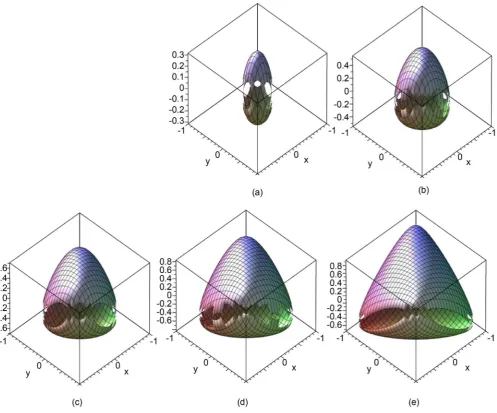
=C in the interior of the

hypercube are shown in Figure 1, for some positive values between 0< <C 1. Instead,

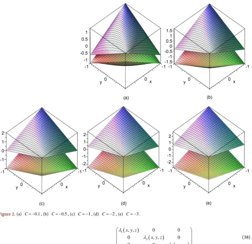
in Figure 2, some surfaces for negative C values are displayed with − < <3 C 0.

The Kummer ΣK surface is given by the condition detρ

( )

r =0, that is

2 2 2

(8)

Figure 1. (a) C=0.9, (b) C=0.7, (c) C=0.5, (d) C=0.3, (e) C=0.1.

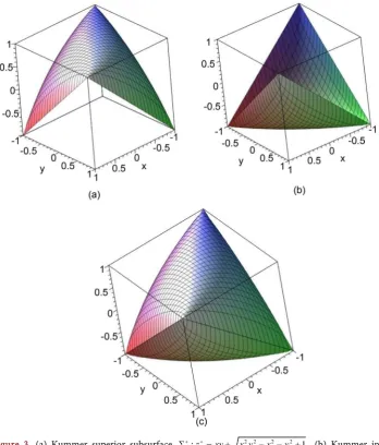
From (36) one found that the Kummer Σ0 subsurface inside the hypercube is given by the parametric equations

(

_,

)

2 2 2 2 ₁

z=z± x y =xy± x y −x −y + (37)

Figure 3 shows the Kummer superior subsurface 0 +

Σ _{given by}z=z+

(

x y,

)

, the Kummer inferior subsurface 0

−

Σ given by z=z−

(

x y,

)

and the complete Kummer subsurface Σ0.

Because Σ0 separates a region with detρ >0 from that with detρ <0 and due to the origin r=

(

0, 0, 0

)

the determinant is one, then inside of Σ₀ the determinant of the ρ matrix must be positive, which is consistent with Figure 1. The region situated between Σ0 and the cube has negative determinant in this case.

[image:8.595.52.550.72.485.2]

(9)

Figure 2. (a) C= −0.1, (b) C= −0.5, (c) C= −1, (d) C= −2, (e) C= −3.

(

)

(

)

(

)

1

2

3

, , 0 0

0 , , 0

0 0 , ,

x y z

λ

 

 

 

(38)

where the three eigenvalues λ ≠1 0, λ ≠2 0 and λ ≠3 0 when r=

(

x y z, ,

)

∉ Σ0. On the Kummer superior subsurface 0

+

Σ _{, the diagonal form of the} ρ_{matrix is}

(

)

(

)

1

2

, 0 0

0 , 0

0 0 0

x y

λ

+

 

 

 

(39)

where

(

)

2 2 2 2 2 2

1

3 1

, 1 8 8 1

2 2

x y x y xy x y x y

[image:9.595.46.556.67.560.2]

(10)

Figure 3. (a) Kummer superior subsurface 2 2 2 2 0:z xy x y x y 1

+ +

Σ = + − − + , (b) Kummer inferior subsurface 2 2 2 2

0:z xy x y x y 1

− −

Σ = − − − + , (c) complete Kummer subsurface Σ0. Note

that the Kummer subsurface Σ0 is closed and its is completely inside the hypercube in this case.

Thus the region between Σ0 and the hypercube has negative ρ determinant for the three

assets system.

and

(

)

2 2 2 2 2 2

2

3 1

, 1 8 8 1

2 2

λ+ _{= −} ₊ ₊ ₋ ₋ ₊ ₍₄₁₎

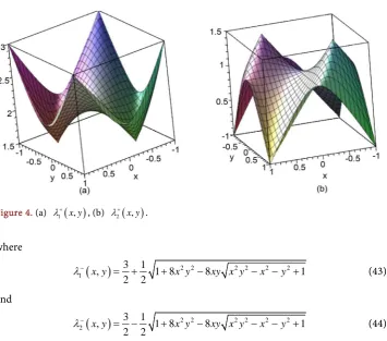
Figure 4 gives the eigenvalues λ1

(

x y,

)

+ _and

₍

₎

2 x y,

λ+ _{as functions of x and y.} For the Kummer inferior subsurface 0

−

Σ , the diagonal form of the ρ matrix is instead

(

)

(

)

1

2

, 0 0

0 , 0

0 0 0

x y

λ

−

 

 

 

[image:10.595.200.549.72.481.2]

(11)

Figure 4. (a) λ1

( )

x y,

+ _{, (b)}

( )

2 x y,

λ+ _.

where

(

)

2 2 2 2 2 2

1

3 1

, 1 8 8 1

2 2

λ− _{= +} ₊ ₋ ₋ ₋ ₊ ₍₄₃₎

and

(

)

2 2 2 2 2 2

2

3 1

, 1 8 8 1

2 2

λ− _{= −} ₊ ₋ ₋ ₋ ₊ ₍₄₄₎

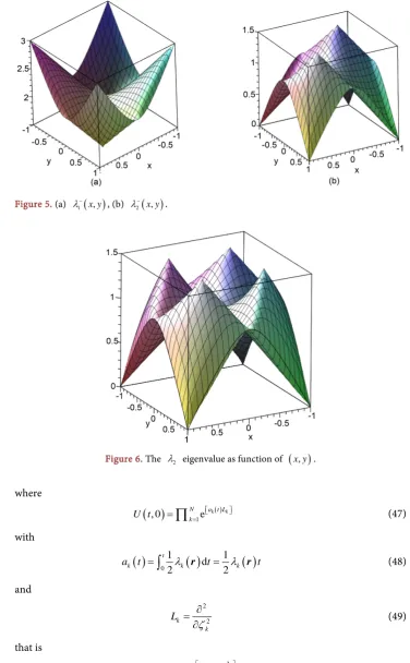
Figure 5 gives the eigenvalues λ1

(

x y,

)

− _and

(

)

2 x y,

λ− _{as functions of x and y.} Note that the eigenvalues λ1

(

x y,

)

+ _and

(

)

1 x y,

λ− _{are always greater than zero, but}

(

)

2 x y,

λ+ _and

(

)

2 x y,

λ− _{are zero for the extreme values of the correlation parameter}

1

x= ± and y= ±1. Figure 6 shows both eigenvalues λ₂+

(

x y,

)

and λ₂−

(

x y,

)

in the same graph. It is possible to see clearly that the λ2

(

x y,

)

proper value becomes equal to zero only for the extreme correlations value cases

(

1,1,1 ,

)

(

1, 1, 1 ,

)

(

1,1, 1 ,

)

(

1, 1,1

)

= = − − = − − = − −

r r r r (45)

which are the vertexes of the Kummer Σ0 subsurface in Figure 3 or the four base points of Figure 6.

Thus, depending on which region of the three dimensional cube the vector r=

(

x y z, ,

)

is lying, the correlation matrix ρ_{has two null eigenvalues, one null eigenvalue or it} can be invertible. Thus the rank of the ρ_{matrix changes when}r moves along the Kummer surface.

5. Pricing, the Wei-Norman Theorem, Propagators and

Σ

K

The problem of pricing the multi-asset option Π_{is now tackled by taking into} account the geometrical properties of the correlation ρ _{matrix analyzed in the} Section 3. In order to do that one needs first to solve the Equation (23). For this, the Wei-Norman theorem [23]-[26] is applied. In this particular case this theorem estab- lishes that the solution of (23) can be writing as

( )

,t U t

( ) (

, 0 , 0

)

[image:11.595.197.553.62.375.2]

(12)

Figure 5. (a) λ1

( )

x y,

− _{, (b)}

( )

2 x y,

λ− _.

Figure 6. The λ2 eigenvalue as function of

( )

x y, .

where

( )

1 , 0 N eakt Lk

k

U t =

∏

₌   (47) with

( )

₀1

( )

1

( )

d

2 2

t

k k k

a t =

∫

λ r t= λ r t (48)

and

2

k k

L ζ ∂ =

∂ (49)

that is

( )

(

)

2

1 2 1

, e , 0

k k t N k

t

λ ζ

 _∂ 

 

 ∂ 

 

=

[image:12.595.179.556.72.681.2]

(13)

by inserting N one dimensional Dirac’s deltas, one can write the above equation as

( )

(

) (

)

2 2 1 2 1 1

, e d , 0

k k

t

N N

m m m

k m

t

λ

ζ _{ζ δ ζ} _ζ

 ∂ 

 

 ∂ 

 

=  = ′ ′  ′

Ψ ζ =

∏

r _

∏ ∫

− _Ψ ζ (51)

or as

( )

,t KΨ

(

, |t ′0

) (

′, 0 d

)

′

Ψ ζ =

_∫

ζ ζ Ψ ζ ζ (52) where the propagator KΨ is defined by

(

)

( ) ( )

₍

₎

2 2 1 2 1

, | 0 e

k k t N N k K t λ ζ _δ  ∂     ∂   

Ψ ′ =

∏

=  − ′ 

r

ζ ζ ζ ζ (53)

with _δ( )N

₍

_{ζ ζ}₋ _′

₎

the N dimensional Dirac’s delta. Now using the Fourier expansion

( )

₍

₎

( )

( ) d e 2π N i N

δ ₋ _′ ₌ ⋅ −′

∫

p pζ ζ

ζ ζ ₍₅₄₎

the propagator can be written finally as the product

(

)

1 ( ) 2 ( )

2 1

d

, | 0 e

2π

k tpk ipk k k

N _k

k p

K_Ψ t ′ = ₌ _ − λ + − ′ _

 

∏ ∫

r ζ ζ

ζ ζ (55)

The Propagator Inside Σ0

When r is inside of Σ0, all eigenvalues λk

( )

r are positive, so the N integrations in

(55) can be performed to give [27][28]

(

)

( )

2

2 1

1

, | 0 e

2π k k k N t k k K t t ζ ζ λ λ ′ − − Ψ =     ′ =    

∏

ζ ζ (56)

or

(

)

( )

( )2 1 2

1 2 1

, | 0 e

2π

N _k _k

k k t N N K t t ζ ζ λ

λ λ λ

= ′ − − Ψ ∑ ′ = 

ζ ζ (57)

By using transformations (15), (16), (17) and (18) one can write the propagator for the option price Π

(

S,τ

)

in the

(

S,τ

)

space as

(

)

(

)

(

)

(

)

( )

(

)

( ) 1 2

1 2 1 2

exp

, | e

2π det t T N N N r T K T

T S S S

ρ τ

τ τ

τ ρ σ σ σ

−     − ₋      Π − − ′ = ′ ′ ′ − S S   α α (58) with

(

)

(

)

2 1 ln 2 , i i i

i i i i

i S r T S S S σ τ σ  _{ }₊ ₋  ₋  _′       ′ = =

α α (59)

(14)

hypercube that verifies det

( )

ρ >0 and have only positive eigenvalues.

6. The Propagator for the Kummer Surface

Σ

K

In this section, an expression for the propagator over the Kummer surface ΣK is

obtained. It is assumed that a region ΣK_NB of ΣK that has NA non zero eigenvalues

and NB =N−NA null eigenvalues. Due to it is on the ΣK surface, the Equation (26)

implies that one of the coordinates of the r vector, is determined by the other M −1 coordinates. These independent coordinates are called x x1, 2,,xM−1. Thus in this section, the vector r is an M dimensional vector that depends on M−1 independent coordinates. In this situation the propagator in (55) gives

(

)

1 ( ) 2 ( ) ( )

2

1 1

d d

, | 0 e e

2π 2π

k k k k k j j j

A tp ip B ip

N k N j

k j

p p

K_Ψ t ′ =  ₌ − λ + ζ ζ− ′ _{ }  ₌ ζ ζ−′ _

 



∏

∫



∏

∫

r

ζ ζ (60)

By performing the integrations

(

)

( )

(

)

2 1 2 1 1 2 e , | 0

2π

N A _k _k

k k B A A t N j j j N N K t t ζ ζ λ

δ ζ ζ

λ λ λ

= ′ − − Ψ = ∑ ′ =

_∏

− ′ 

ζ ζ (61)

If the N dimensional vector ζ _{is separated in two parts as}

1 1 1 ₁ A A A B N N A N B N N ζ ζ ζ ζ ζ _ζ ζ ζ +    _{ } _         _ _ _ __{  }   =_ _=_ _{ }= _         _ _     _ _ _  _ _ _       ζ

ζ _ζ (62)

the above propagator can be written in a more compact form as

(

)

( )

( ) ( ) ( )

₍

₎

1 2 1

, | 0 e

2π det

t

A A A A A

B A D N t B B N A K t t D δ − ′ ′ − −

Ψ ′ = − ′

ζ ζ ζ ζ

ζ ζ ζ ζ (63)

where 1 2 0 0 0 0 0 0 A N A D λ λ λ       =              (64)

is the reduced diagonal ρ matrix on the Kummer surface ΣK. If one separates the

vector χ_{in A and B components as}

A B   =     χ χ

χ (65)

then relation (20) induces the transformation

1 1

A AA AB A

B BA BB B

U U U U − − − −       =            ζ χ

(15)

where 1

AA U− , 1

AB U− , 1

BA

U− and 1

BB

U− are the matrices that result from sectioning U−1

into A and B components.

The quadratic term in the exponential of (61) can be expressed in the χA and χB

components as

(

)

(

)

(

)

(

) (

)

(

)

(

)

(

) (

)

(

)

1

1 1 1 1 1 1

t

A A A A A

t t

A A AA A AA A A B B AB A AA A A

t t

A A AA A AB B B B B AB A AB B B

D

U D U U D U

− − − − − − − − − − − − − ′ ′ − −     ′ ′ ′ ′ = − _ _ − + − _ _ −     ′ ′ ′ ′ + − _ _ − + − _ _ −

ζ ζ ζ ζ

χ χ χ χ χ χ χ χ

(67)

Now, from (66)

(

)

1

(

)

1

(

)

B B UBA A A UBB B B

− −

′ ′ ′

− = − + −

ζ ζ χ χ χ χ (68)

The Dirac’s delta in (63) implies that

(

)

(

)

1 1

0=U_BA− χ_A−χ′_A +U_BB− χ_B−χ′_B (69) The above equation permits writing the vector

(

χB−χB′

)

in terms of

(

χA−χA′

)

as

(

)

1

(

)

B B U UBB BA A A

−

′ ′

− = − −

χ χ χ χ ₍₇₀₎

replacing in (67) one can write the quadratic term as

(

)

1

(

) (

)

1

(

)

K

t t

A A DA A A A A ρ A A

− −

Σ

′ ′ ′ ′

− − = − −

ζ ζ ζ ζ χ χ χ χ (71)

where 1

K ρ−

Σ is defined by

1 1 1 1 1 1 1 1

1 1 1 1 1 1 1 1 1

K

t t

AA A AA AB BB BA A AA

t t

AA A AB BB BA AB BB BA A AB BB BA

U D U U U U D U

U D U U U U U U D U U U

ρ− − − − − − − −

Σ

− − − − − − − − −

   

=_ _ +_ _

   

+_ _ +_ _ (72)

From (66)

dζ =dζ ζAd B =dχ χAd B =dχ (73)

Using (68) and (71) in (52), the option price can be written as

(

)

( ) ( )

( )

(

₍

₎

₍

₎

)

₍

₎

1 2 1 1 e

, , , , 0 d d

2π det

t

A A _K A A

B

A

t

N

A B _N BA A A BB B B A B A B

A

t U U

t D ρ δ − Σ ′ ′ − − − _′ − _′ _′ _′ _′ _′

Ψ =

_∫

− + − Ψ

χ χ χ χ

χ χ χ χ χ χ χ χ χ χ ₍₇₄₎

Integrating over dχB′ gives

( )

(

)

( ) ( )

( )

(

)

1 2 1 e 1

, , , , 0 d

det 2π det

t

A A _K A A

A

t

A B _N A B A

BB A t U t D ρ− Σ ′ ′ − − − ′ ′ ′

Ψ_r =

_∫

Ψ

χ χ χ χ

χ χ χ χ χ ₍₇₅₎

where χB′ must be evaluated from (70) in terms of χB and

(

χA−χA′

)

as

(

)

B′ = B+γ A− A′

χ χ χ χ (76)

where the rectangular NB×NA matrix γ is defined by

1

BB BA U U

(16)

It must be noted that 1

U− , the eigenvalues λi, and the rectangular matrix γ are

functions of the vector r that lies on the null surface Σ_K. Thus the option price is also a function of r. Using (15), (16), (17) and (18) one can write the option price in the

(

S,τ

)

space as Π_{( )}_r

(

S,τ

)

and is given by

( )

(

)

( ) ( ) ( )

(

)

(

)

( )

(

)

1 2 1 1 1

, , d

e e

, ,

det

2π det

t

A _K A

A

A A

T r T

A B A

A B _N

N N BB A T S S U T D ρ τ τ τ σ σ τ − Σ − − − − ′ ′ Ψ ′ Π = ′ ′ −

∫

r

S S S

S S

 

α α

(78)

where the components of the α are given by

(

)

2

1 ln

2

, 1, ,

j A j j A j A A j S r T S j N σ τ α σ  _{ }₊ ₋  ₋  _′  _ _  

= =  (79)

and the components of the vector SB′ are given in terms of SA, SA′ and SB

according to ( ) 2 2 1 1 1 2 2

1 e , 1, ,

N

i A _i

ij _i _ij _j

j _j _j

A

r r T

j N

i i A

B B j j B

A

S

S S i N

S

σ _γ _σ

σ γ σ τ

σ _σ = _ _ _ _ − + − − _ _ _ _     = ∑       ′ = _ _ _ _ = ′      

∏

 (80)

with γij the components of the rectangular matrix γ

1 _, _1, _, _, _1, _,

ij U UBB BA _ij i NB j NA

γ ₌_ − _ ₌ ₌

    (81)

When r moves over the Kummer surface Σ_K, the rank of the ρ matrix can change, so the dimensions of NA and NB =N−NA also change, but Equation (78)

is always valid.

7. The Propagator Outside

Σ

0

When the vector r is lying outside the Kummer subsurface Σ0, there are regions where the determinant of the correlation matrix is negative. This implies that the propagator given in (58) becomes complex. But, worse than that, in this case one of the eigenvalues λk is negative, so the propagator given in (57) generates an exponential

growth in the associated ζk coordinate. Then the convolution in (52) is not well

defined. Thus, one cannot price the option in regions outside the Kummer subsurface

0

Σ _{that have negative} ρ determinant.

8. Conclusions and Further Research

In this research, the existence of the solution of the multi-asset Black-Scholes model has been analyzed in detail. It has been shown that the correlation parameter space, which is equivalent to an N dimensional hypercube, limits the existence of a valid solution for the multi-asset Black-Scholes model. Particularly, it has been demonstrated that inside of this hypercube there is a surface, called the Kummer surface ΣK, where the

(17)

assets and its implied geometry has been studied in detail when the determinant of the correlation matrix is zero. Finally, by using the Wei-Norman theorem, the propagator over the variable rank surface ΣK for the general N asset case has been computed,

which is applicable over all the Kummer surface, whatever be the rank of the ρ matrix. This formulation corrects the past solution of this problem and its extensions. As future research, most of the papers related to the multi-asset Black-Scholes model must be revisited in line of our results, as well as others where it is implicitly assumed that a well behaved multivariate Gaussian distribution must exist, as is the case of the stochastic volatility family (see for instance [29][30]).

References

[1] Black, F. and Scholes, M. (1973) The Pricing of Options and Corporate Liabilities. Journal of

Political Economy, 8, 637-654. http://dx.doi.org/10.1086/260062

[2] Merton, R.C. (1973) Theory of Rational Option Pricing. Bell Journal of Economics and

Management Science, 4, 141-183. http://dx.doi.org/10.2307/3003143

[3] Paul, W. (2000) Paul Wilmott on Quantitative Finance. Wiley, Hoboken. [4] Jim, G. (2006) The Volatility Surface. Wiley, Hoboken.

[5] Hull, J. and White, A. (1987) The Pricing of Options on Assets with Stochastic Volatilities.

The Journal of Finance, 42, 281-300.

[6] Chen, L. (1996) Stochastic Mean and Stochastic Volatility: A Three-Factor Model of the Term Structure of Interest Rates and Its Application to the Pricing of Interest Rate Deriva-tives. Financial Markets, Institutions, and Instruments, 5, 1-88.

[7] Tomas, B. (2009) Arbitrage Theory in Continuous Time. 3rd Edition, Oxford Finance Se-ries, Oxford.

[8] Margrabe, W. (1978) The Value of an Option to Exchange One Asset for Another. The

Journal of Finance, 33, 177-186. http://dx.doi.org/10.1111/j.1540-6261.1978.tb03397.x

[9] Stulz, R.M. (1982) Options on the Minimum or the Maximum of Two Risky Assets: Analy-sis and Applications. Journal of Financial Economics, 10, 161-185.

http://dx.doi.org/10.1016/0304-405X(82)90011-3

[10]Johnson, H. (1987) Options on the Maximum or the Minimum of Several Asset. Journal of

Financial and Quantitative Analysis, 22, 277-283. http://dx.doi.org/10.2307/2330963

[11]Reiner, E. (1992) Quanto Mechanics, from Black-Scholes to Black Holes: New Frontiers in Options. RISK Books, London, 147-154.

[12]Shimko, D.C. (1994) Options on Futures Spreads: Hedging, Speculation, and Valuation.

Journal of Futures Markets, 14, 183-213. http://dx.doi.org/10.1002/fut.3990140206

[13]Embrechts, P., McNeil, A. and Straumann, D. (2002) Correlation and Dependence in Risk Management: Properties and Pitfalls. Risk Management: Value at Risk and Beyond. 1st Edi-tion, Cambridge University Press, Cambridge, 176-223.

[14]Boyer, B.H., Gibson, M.S. and Loretan, M. (1997) Pitfalls in Tests for Changes in Correla-tions. Board of Governors of the Federal Reserve System, 597.

https://www.federalreserve.gov/pubs/ifdp/1997/597/

[15]Patton, A.J. (2004) On the Out-of-Sample Importance of Skewness and Asymmetric De-pendence for Asset Allocation. Journal of Financial Econometrics, 2, 130-168.

(18)

[16]Nielsen, B.F., Skavhaug, O. and Tveito, A. (2008) Penalty Methods for the Numerical Solu-tion of American Multi-Asset OpSolu-tion Problems. Journal of Computational and Applied

Mathematics, 222, 3-16. http://dx.doi.org/10.1016/j.cam.2007.10.041

[17]Persson, J. and von Sydow, L. (2008) Pricing European Multi-asset Options Using a Space- Time Adaptive FD-Method. Technical Report 2003-059, Department of Information Tech-nology, Uppsala University, Uppsala.

[18]Mehrdoust, F., Fathi, K. and Rahimi, A.A. (2013) Numerical Simulation for Multi-Asset Derivatives Pricing under Black-Scholes Model. Chiang Mai Journal of Science, 40, 725-735. [19]Kummer, E. (1975) Collected Papers. Vol 2, Springer-Verlag, Berlin.

[20]Hudson, R.W. (1905) Kummer’s Quartic Surface. Cambridge University Press, Cambridge. [21]Labs, O. (2006) Hypersurfaces with Many Singularities. PhD Thesis, Johannes Gutenberg

Universität,Mainz.

[22]Dolgachev, I.V. (2012) Classical Algebraic Geometry: A Modern View. Cambridge Univer-sity Press, Cambridge. http://dx.doi.org/10.1017/CBO9781139084437

[23]Wei, J. and Norman, E. (1963) Lie Algebraic Solution of Linear Differential Equations.

Journal of Mathematical Physics, 4, 575-581. http://dx.doi.org/10.1063/1.1703993

[24]Lo, C.F. and Hui, C.H. (2002) Pricing Multi-Asset Financial Derivatives with Time-Depen- dent Parameters-Lie Algebraic Approach. International Journal of Mathematics and

Ma-thematical Sciences, 32, 401-410. http://dx.doi.org/10.1155/S016117120211101X

[25]Martin, J.F.P. (1968) On the Exponential Representation of Solutions of Linear Differential Equations. Journal of Differential Equations, 4, 257-279.

http://dx.doi.org/10.1016/0022-0396(68)90038-7

[26]Charzyński, S. and Kuś, M. (2013) Wei-Norman Equations for a Unitary Evolution. Journal

of Physics A: Mathematical and Theoretical, 4, Article ID: 265208.

http://dx.doi.org/10.1088/1751-8113/46/26/265208

[27]Kleinert, H. (2006) Path Integrals in Quantum Mechanics, Statistics, Polymer Physics, and Financial Markets. 4th Edition, World Scientific, Singapore. http://dx.doi.org/10.1142/6223 [28]Chaichian, M. and Demichev, A. (2001) Path Integrals in Physics. Vol. 1, IOP Publishing,

Bristol.

[29]Contreras, M. (2015) Stochastic Volatility Models at ρ= ±1 as a Second Class Constrained

Hamiltonian Systems. Physica A, 405, 289-302. http://dx.doi.org/10.1016/j.physa.2014.03.030

[30]Contreras, M. and Hojman, S. (2014) Option Pricing, Stochastic Volatility, Singular Dy-namics and Path Integrals. Physica A, 393, 391-403.

(19)

Submit or recommend next manuscript to SCIRP and we will provide best service for you:

Accepting pre-submission inquiries through Email, Facebook, LinkedIn, Twitter, etc. A wide selection of journals (inclusive of 9 subjects, more than 200 journals)

Providing 24-hour high-quality service User-friendly online submission system Fair and swift peer-review system

Efficient typesetting and proofreading procedure

Display of the result of downloads and visits, as well as the number of cited articles Maximum dissemination of your research work

Submit your manuscript at: http://papersubmission.scirp.org/