Image Recognition using Coefficient of Correlation and Structural SIMilarity Index in Uncontrolled Environment

Image Recognition using Coefficient of Correlation and

Structural SIMilarity Index in Uncontrolled Environment

Avneet Kaur

, Lakhwinder Kaur

and Savita Gupta

Department University College of Engineering (UCOE), Punjabi University, Patiala, Punjab (India) ,2

Department University Institute of Engineering (UIET), Panjab University, Chandigarh (India)

ABSTRACT

The goal of this paper is to analyse and improve the performance of metrics like Coefficient of Correlation (CoC) and Structural Similarity Index (SSIM) for image recognition in real-time environment. The main novelties of the methods are; it can work under uncontrolled environment and no need to store multiple copies of the same image at different orientations. The values of CoC and SSIM get changed if images are rotated or flipped or captured under bad/highly illuminated conditions. To increase the recognition accuracy, the input test image is pre-processed. First, discrete wavelet transform is applied to recognize the image captured under bad illuminated and dull lightning conditions. Second, to make the method rotation invariant, the test image is compared against the stored database image without and with rotations in the horizontal, vertical, diagonal, reverse diagonal and flipped directions. The image recognition performance is evaluated using the Recognition Rate and Rejection Rate. The results indicate that recognition performance of Correlation Coefficient and SSIM gets improved with rotations and discrete wavelet transform. Also it was observed that CoC with proposed modifications yield better results as compared to state of the art enhanced Principal Component Analysis and Enhanced Subspace Linear Discriminant Analysis.

Keywords—Image Recognition, Discrete Wavelet Transforms, Correlation Coefficient, Structural Similarity Index Metrics.

1.

INTRODUCTION

In image recognition applications we often need to find the similarity between two images i.e. between test image and its equivalent training database image. Image recognition has become of great interest over the past decades because of its potential applications in many fields, such as Optical Character Recognition (OCR), identity authentication, human-computer interfacing, and surveillance. A wide variety of recognition methods for image recognition, especially for face image recognition are reported in the literature [1]. In this survey various methods for image recognition are categorized as Holistic methods [2-4], Feature-based methods [5-7], Hybrid methods [8]. In 2012, Avneet et al. have improved the performance of well known image recognition methods;

Principal Component Analysis (PCA) and Subspace Linear Discriminant Analysis (LDA) [9] by usingDiscrete Wavelet Transform (DWT) and rotations. With suggested improvements [9], the methods operated well in controlled as well as in uncontrolled environments. Image recognition in well-controlled environments means that the imaging conditions are fixed for both the trainee as well as the probe images and is relatively mature field of research [10]. Research in uncontrolled environments is much less mature and the results from well-controlled environments cannot be assumed to hold in uncontrolled environments.

Recognition in controlled environments can be time and cost intensive and can be impractical to use in real world use [10]. As part of this research, main emphasis is on the assessment of suitability of image recognition systems in uncontrolled environment and their ability to use in real-world. The metrics coefficient of correlation (CoC) measure the degree of correlation between two images and SSIM can measure structural similarity between two images [23]. In this paper, these simple metrics, CoC and SSIM are used for image recognition, which are often used as image quality measures. The paper is organized as follows. In next section, we have discussed the DWT which is used as pre-processing step for the image recognition methods. Section 3 includes the discussions about Correlation Coefficient and SSIM used for image recognition. In Section 4, discussed the database used for the experimental purposes and experimental results. Finally, section 5 contains conclusions drawn from the experimental results.

2.

DISCRETE

WAVELET

TRANSFORMS

(DWT)

The wavelet transform concentrates the energy of the image signals into a small number of wavelet coefficients. It has good time-frequency localization property [11, 24]. The fundamental idea behind wavelets is to analyse signal according to scale. It was developed as an alternative to the short time Fourier to overcome problems related to its frequency and time resolution properties [12] [13]. Wavelet transform decomposes a signal into a set of basic functions. These basic functions are obtained from a mother wavelet by translation and dilation [14].

where a and b are both real numbers which quantify the scaling

and translation operations respectively. The advantage of DWT over DFT and DCT is that DWT performs a multi-resolution analysis of signal with localization in both time andfrequency. Also, functions with discontinuities and with sharp spikes require fewer wavelet basis vectors in the wavelet domain than sine-cosine basis vectors to achieve a comparable approximation [15].

Figure 1: Process of decomposing an image [13] [14]

low-frequency component in the horizontal direction and high-frequency component in the vertical direction [17].

Figure: 2 (a) Original Image (b) After 1-level wavelet transform

3.

IMAGE

RECOGNITION

METHODS

3.1 Coefficient of Correlation(CoC)

Correlation is a method for establishing the degree of probability that a linear relationship exists between two measured quantities. In 1895, Karl Pearson defined the Pearson product-moment correlation coefficient r. Pearson’s correlation coefficient, r, was the first formal correlation measure and is widely used in statistical analysis, pattern recognition and image processing. For monochrome digital images, the Pearson’s correlation coefficient is defined as [18]:

where, xi and yi are intensity values of i th

pixel in 1st and 2nd image respectively.

Also, xm and ym are mean intensity values of 1 st

and 2nd image respectively.

The correlation coefficient has the value r =1 if the two images are absolutely identical, r= 0 if they are completely uncorrelated and r= -1 if they are completely anti-correlated [19].

The Pearson product-moment correlation coefficient is a dimensionless index, which is invariant to linear transformations of either variable [18].

 Benefits of Correlation Coefficient:

-It condenses the comparison of two 2-D images down to a single scalar value, r [19].

-It is completely invariant to linear transformations of x and y. So, r is insensitive (within limits) to uniform variations in brightness or contrast across an image [18] [19].

 Limitations of Correlation Coefficient:

- It is computationally intensive. This limits its usefulness for image registration [19].

-It is extremely sensitive to the image skewing, pincushioning and vignetting that inevitably occurs in imaging systems [19]. - It can be undefined in some practical applications -- due to the division by zero -- if one of the test images has constant, uniform intensity [19].

3.2. Structure Similarity Index Metrics (SSIM)

It is observed that natural image signals are highly structured i.e., the image signal samples exhibit strong dependencies amongst themselves, especially when they are spatially proximate. These dependencies carry important information about the structure of the objects in the visual scene [20]. SSIM is full-reference image quality assessment methods; the quality of a test image is evaluated by comparing it with a reference image that is assumed to have perfect quality [21]. The goal of image quality assessment research is to design methods that quantify the strength of the perceptual similarity (or difference) between the test and the reference images. So,

this SSIM values can be used to measure the similarity between the structure of test image and stored database training images for recognizing the images. Brief overview of this similarity measurement system is as follows [20]:

Figure: 3 Diagram of the proposed similarity measurement system [21].

Suppose x and y are two non-negative image signals, which can either be continuous signals or discrete signals represented

as and ,

respectively, where i is the sample index and N is the number of signal samples (pixels). The purpose of the system is to provide a similarity measure between them [20].

To measure similarity between them the task is separated into three comparisons: luminance, contrast and structure. First, the luminance of each signal is compared. The mean intensity of discrete signal is as follow [20]:

The luminance comparison function is then a function of and [20]:

Second, we remove the mean intensity from the signal. The resulting signal corresponds to the projection of vector x

onto the hyper plane of

The standard deviation is used to estimate signal contrast. An unbiased estimate in discrete form is given by [20]:

The contrast comparison c(x, y) is then the comparison of

and :

Third, the signal is normalized by its own standard deviation; so that the two signals are being compared have unit standard deviation. The structure comparison s (x, y) is conducted on these normalized signals [20]:

Finally, the three components are combined to yield an overall similarity measure [20]:

Similarity measure should satisfy the following conditions [20]:

1. Symmetry: i.e. by exchanging the order of input signals similarity measurement should not be affected.

2. Boundedness: as an upper bound can serve as an indication of how close the two signals are to being perfectly identical.

3. Unique maximum: if and only if x = y The luminance comparison function is [20]:

where the constant is included to avoid instability when

is very close to zero. Its chosen value is:

where L is the dynamic range of the pixel values and is a small constant.

The contrast comparison function will be [20]:

where is non-negative constant having value:

and satisfies .

, by default

Structure comparison is conducted after luminance subtraction and contrast normalization. Thus, structure comparison function as follows [20]:

Finally, by combining eqn (10), (12), (14) Structural SIMilarity (SSIM) index between two image signals x and y is [20]:

where and are parameters used to adjust the relative importance of the three components. To simplify the expression, set and The SSIM index in specific form will be [20]:

Mean SSIM (MSSIM) index to evaluate the overall image quality can be given [21]:

where X and Y are the reference and the distorted images, respectively; xj and yjare the image contents at the jth local

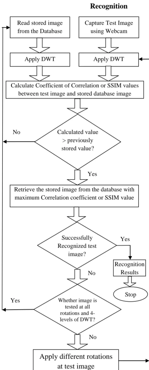
window; and M is the number of local windows in the image. 3.3. Basic steps of proposed method

Step 1: Read the image from the stored database and apply DWT to get LL subband for comparison.

Step 2: Then capture the test image using the MATLAB’s Image Acquisition Toolbox.

Step 3: Apply 1- level DWT on the test image

Step 4: Calculate the Correlation Coefficient or SSIM values (depending upon the method used for recognition) between LL subband of test image and that of stored database image. Step 5: Check whether this calculated value is more than the previously stored value.

(a) If it is less than previously stored value i.e. (Calculated Value < Previous Value), then go to step 6(c).

Step 6: Check for successful recognition.

(a) If the test image is recognized successfully then read recognized image and STOP.

(b) If image is tested at different rotations and 1 to 4-levels of DWT then goto step 1.

(c) Else goto step 3 to repeat the same procedure at different rotations and 1 to 4 levels of DWT decomposition until we get satisfied results.

Basic steps of the proposed procedure are shown in fig 5.

4.

EXPERIMENTAL

RESULTS

AND

CONCLUSIONS

4.1. Image Database Used

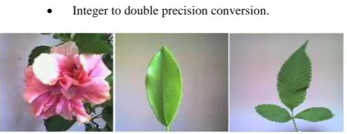
The training dataset used in the experiments consists of the images of three different subjects, which are human faces, plant leaf images and flower images (figure 4). The entire trainees as well as the test images are captured in the real-time environment with the help of MATLAB software’s Image Acquisition Toolbox. Using it, we captured images through CyberLink Web Camera Filter having resolution 160x120 in RGB color space.

Pre-processing of images includes following steps:

 Resize images to size of 120x120.

 Conversion of images from RGB color space to gray scale.

 Integer to double precision conversion.

4.2. Results and discussions

The performance of all the image recognition methods is compared quantitatively in terms of metrics Recognition Rate and Rejection Rate given below [22]:

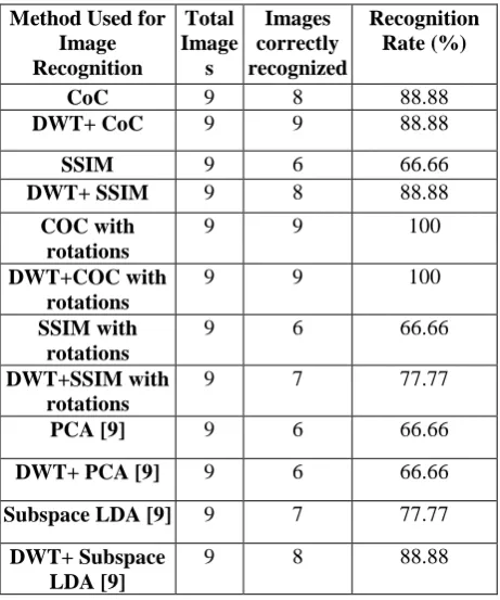
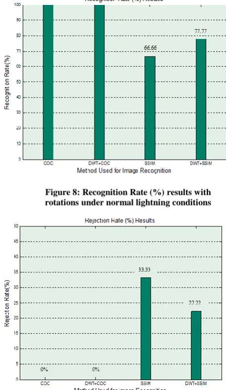
From the Table I , Figure 6 and Figure 7, it is concluded that Correlation Coefficient with and without DWT has high overall recognition rate and low rejection rate as compared to SSIM. However, applying DWT in conjunction with SSIM improves the performance. Figure 8 and Figure 9, revels that when rotations are used in conjunction with Correlation Coefficient then it gives maximum overall recognition rate.

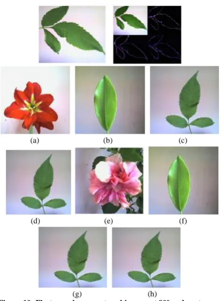
Further, to show the impact of rotations, images are captured at different orientations and image recognition algorithms with and without rotations are applied. The figures 10 - 12, show that simple CoC and SSIM fails to recognize images captured at rotations; 90º, 180º and 270º respectively, but with the application of rotation on captured image they recognize test image. Figure 13, reveals that due to moderate illumination effect CoC and SSIM yield wrong results, but with the application of 1-level DWT, CoC and SSIM recognizes correct

images. In case when test image is captured under highly illuminated conditions, CoC with level-1 DWT fails to recognize it. So, level-2 DWT is used to successfully recognize highly illuminated test image (see Figure 14). From Figure 15, it is clear that due to dull lightning conditions, CoC and SSIM yields wrong results, but with application of 4-level DWT they recognizes correct images. This is due to fact that with 4-level DWT decomposition, it concentrates more energy in the LL subband, hence recognizes dull images.

Table I: Recognition accuracy of image recognition different methods under normal lightning conditions

Method Used for Image Recognition Total Image s Images correctly recognized Recognition Rate (%)

CoC 9 8 88.88

DWT+ CoC 9 9 88.88

SSIM 9 6 66.66

DWT+ SSIM 9 8 88.88

COC with rotations

9 9 100

DWT+COC with rotations

9 9 100

SSIM with rotations

9 6 66.66

DWT+SSIM with rotations

9 7 77.77

PCA [9] 9 6 66.66

DWT+ PCA [9] 9 6 66.66

Subspace LDA [9] 9 7 77.77

DWT+ Subspace LDA [9]

9 8 88.88

5. CONCLUSION

From the results, it is clear that all the recognition methods with proposed modifications yield satisfactory results in the uncontrolled environments. Under normal lightning conditions, recognition accuracy of Correlation Coefficients when used with and without DWT on the rotated test images gives the best results as compared to SSIM, PCA and LDA [9]. However, the performance of all the methods gets improved for uncontrolled environment with the application of rotations and DWT. For highly illuminated images, 2 levels of wavelet decomposition are sufficient, whereas for dull images 4-level decompositions are sufficient. The CoC yields the best results among all the methods. The novelties of the method are reduced data set for comparison as only LL subband is compared, and methods are rotation invariant (no need to store multiple copies of the same image). The algorithms have been on tested on plant images; same can be tested on human faces also. These methods can be used for real-world applications with a little attention.

6. REFERENCES

[1] W.Zhao, R.Chellappa, P. J. Phillips, A. Rosenfeld, “Face Recognition: A Literature Survey”, ACM Computing Surveys, Vol. 35, No. 4, December 2003, pp. 399–458 [2] M.Turk, A.Pentland, “Eigenfaces for Recognition”,

Journal of Cognitive Neuroscience, Vol. 3, No. 1, 1991, pp. 71-86

[3] W.Zhao, R.Chellappa, A.Krishnaswamy, “Discriminant Analysis of Principal Components for Face Recognition”, Proceedings of the 3rd IEEE International Conference on face and Gesture Recognition, FG’98, 14-16 April 1998,Nara,Japan,pp.336-341

[4] P. N. Belhumeur, J. P. Hespanha, and D.J. Kriegman “Eigenfaces vs. Fisherfaces: Recognition using Class Specific Linear Projection”, IEEETransaction on Pattern Analysis Machine Intelligence (PAMI), Vol.19, 1997, pp. 711–720

[5] T.Kanade, “Computer recognition of human faces”, Birkhauser, Basel, Switzerland, and Stuttgart, Germany,1977

[6] A. V. Nefian, M.H. Hayes III, “Hidden Markov models for face recognition”, Proceedings of IEEE International Conference on Acoustics, Speech and Signal Processing,12-15 May 1998,Vol.5,pp.2721-2724 [7] L.Wiskott, J.M. Fellous, N. Kruger, C. Malsburg, “ Face

Recognition by Elastic Bunch Graph Matching”, IEEE Transaction on Pattern Analysis Machine Intelligence (PAMI), Vol.19, 1997, pp. 775–779

[8] J. Huang, B. Heisele, V. Blanz, “Component-based Face Recognition with 3D Morphable Models”, Proceedings of the 4th International Conference on Audio and Video Based Biometric Person Authentication (AVBPA), 09-11 June 2003, Guildford, UK, pp. 27-34

[9] A. Kaur, L. Kaur and Savita Gupta, “Performance Improvement of LDA and PCA algorithms for Image Recognition”, Proceedings of International Conference on Electrical Engineering and Computer Science (ICEECS), June 2012

[10] Charles Schmitt, Sean Maher, “The Evaluation and Optimization of Face Recognition Performance Using Experimental Design and Synthetic Images”, A Research Report prepared by RTI International-Institute of Homeland Security Solutions , U.S.A., June 2011

[11] SHI Dongcheng, JIANG Jieqing, “The Method of Facial Expression Recognition Based on DWT-PCA/LDA”, Proceedings of IEEE 3rd International Congress on Image and Signal Processing (CISP), 16-18 October 2010, Yantai, Vol.4, pp.1970-1974

[12] Kamarul Hawari Ghazali, Mohd. Marzuki Mustafa, Aini Hussain, “Image Classification using Two Dimensional Discrete Wavelet Transform”, Proceedings of International Conference on Instrumentation, Control & Automation (ICA),20-22 October 2009, Bandung, Indonesia,pp.71-74

[13] L. Kaur and Savita Gupta, “Wavelet based compression using Daubechies filter”, National Conf. on Communication at IIT Bombay, 2002

Proceedings of the IEEE Pacific-Asia Conference on Knowledge Engineering and Software Engineering (KESE’09), 19-20 December 2009, Shenzhen pp.136-138 [15] Paul Nicholl, Abbes Amira, Djamel Bouchaffra

“Multiresolution Hybrid Approaches for Automated Face Recognition”, Proceedings of the IEEE 2nd NASA/ESA Conference, 5-8 August 2007, Edinburgh.pp.89-96 [16] Meihua Wang, Hong Jiang and Ying Li, “Face

Recognition based on DWT/DCT and SVM”, Proceedings of the IEEE International Conference on Computer Application and System Modeling (ICCASM), 22-24 October 2010, Taiyuan,Vol.3, pp.V3-507-V3-510 [17] Yee Wan Wong, Kah Phooi Seng, Li-Minn Ang,

“M-Band Wavelet Transform in Face Recognition System”, Proceedings of IEEE 5th International Conference on Electrical Engineering/Electronics, Computer, Telecommunications and Information Technology (ECTI) Conference,14-17 May 2008, Krabi ,Vol.1, pp.453-458 [18] J.L.Rodgers, W.A. Nicewander, “Thirteen Ways to Look

at the Correlation Coefficient”, The American Statistician, February 1988, Vol. 42, No. 1, pp.59-66

[19] Eugene K . Jen, Roger G.Johnston, “The Ineffectiveness of Correlation Coefficient for Image Comparisons”, Research Paper prepared by Vulnerability Assessment Team, Los Alamos National Laboratory, New Mexico [20] Zhou Wang, Alan C. Bovik and Hamid R. Sheikh,

“Structural Similarity Based Image Quality Assessment”, Digital Video Image Quality and Perceptual Coding, Chap 7, 2005

[21] Z. Wang, A. Bovik, H. Sheikh, E. Simoncelli “Image Quality Assessment: From Error Visibility to Structural Similarity”, Proceedings of IEEE Transactions on Image Processing, Vol.13, No.4, April 2004,pp. 600-612 [22] Chun Lei He, Louisa Lam, Ching Y. Suen, “A Novel

Rejection Measurement in Handwritten Numeral Recognition Based on Linear Discriminant Analysis”, Proceedings of IEEE 10th International Conference on Document Analysis and Recognition, 2009,pp.451-455. [23] S. Gupta, L. Kaur, R.C. Chauhan and S. C. Saxena, “A

Versatile Technique for Visual Enhancement of Medical Ultrasound Images”, Elsevier jr. of digital signal processing, vol. 17, pp. 542-560, 2007.

[24] L. Kaur, R.C. Chauhan and S. C. Saxena, “Joint Thresholding and Quantizer Selection for Compression of Medical Ultrasound Images in the Wavelet Domain”, Taylor & Francis Jr. of Medical Engg. and Technology (JMET), vol. 30, no. 1, pp. 17-24, Jan-Feb 2k6.

No Yes

Whether image is tested at all rotations and 4-levels of DWT?

Apply different rotations

at test image

Capture Test Image using Webcam Read stored image

from the Database

Apply DWT Apply DWT

Calculate Coefficient of Correlation or SSIM values between test image and stored database image

Retrieve the stored image from the database with maximum Correlation coefficient or SSIM value

Successfully Recognized test

image?

Recognition

Calculated value > previously stored value?

No

Yes

Recognition Results

Stop Yes

Figure 9: Rejection Rate (%) Results with rotations under normal lightning conditions

Figure 8: Recognition Rate (%) results with rotations under normal lightning conditions

Figure 7: Rejection Rate (%) Results under normal lightning conditions

(a) (b) (c)

(d) (e) (f)

(g) (h)

Figure 10: First row shows captured images at 90º and next rows shows the recognized image from the database by (a) CoC, (b)

DWT + CoC,

(c) CoC with rotations, (d) DWT + CoC with rotations, (e) SSIM, (f) DWT + SSIM, (g) SSIM with rotations, and (h) DWT+SSIM

with rotations .

(a) (b) (c)

(d) (e) (f)

(g) (h)

Figure 11: First row shows captured images at 180º and next rows shows the recognized image from the database by (a) CoC, (b)

DWT + CoC,

(c) CoC with rotations, (d) DWT + CoC with rotations, (e) SSIM, (f) DWT + SSIM, (g) SSIM with rotations, and (h) DWT+SSIM

with rotations .

(a) (b) (c)

(d) (e) (f)

(g) (h)

Figure 12: First row shows captured images at 270º and next rows shows the recognized image from the database by (a) CoC, (b)

DWT + CoC,

(c) CoC with rotations, (d) DWT + CoC with rotations, (e) SSIM, (f) DWT + SSIM, (g) SSIM with rotations, and (h) DWT+SSIM

with rotations .

(a) (b) (c)

(d) (e)

Figure 13: (a) shows captured image, (b) shows output of CoC, this is due to illumination problem while capturing image , (c) output of “1-level DWT+ Correlation Coefficient”, (d) output of

SSIM, and (e) output of “level-1 DWT+SSIM”.

(a) (b) (c)

(d) (e)

Figure 14: (a) shows captured image in highly illuminated lighting conditions, (b) shows output of CoC, (c) output of “level-2 DWT+ Correlation Coefficient”, (d) output of SSIM and (e) output of

level-2 DWT+SSIM

(a) (b) (c)

(d) (e)

Figure 15: (a) shows captured image, (b) shows output of Correlation Coefficient due to dull lighting conditions while capturing image, (c) output of “4-level DWT+ CoC”, (d) output of